2020/09/28

keras IMDB 情緒分析 setiment analysis

keras IMDB

情緒分析 setiment analysis 又稱為意見探勘 opinionmining,是以自然語言處理、文字分析的方法,找出作者在某些話題的態度、情感、評價或情緒。可讓廠商提早得知客戶對公司或產品的觀感。

IMDb: Internet Movie Database是線上電影資料庫,始於 1990 年,1998 年起,成為 amazon 旗下的網站,收錄了 4百多萬筆作品資料。

IMDb 資料及共有 50000 筆影評文字,分訓練與測試資料各 25000 筆,每一筆資料都被標記為「正面評價」或「負面評價」

keras 處理 IMDb 的步驟

Step 1. 讀取資料集

訓練資料

​ train_text (文字):0~12499 筆:正面評價文字,12500~24999 筆:負面評價文字

​ y_train(標籤):0~12499 筆:正面評價都是 1,12500~24999 筆:負面評價,都是 0

測試資料

​ test_text (文字):0~12499 筆:正面評價文字,12500~24999 筆:負面評價文字

​ y_test(標籤):0~12499 筆:正面評價都是 1,12500~24999 筆:負面評價,都是 0

Step 2. 建立 token

​ 因為深度學習模型只能接受數字,必須將影評文字,轉換為數字 list。翻譯前,要先製作字典。keras 提供 Tokenizer module,就是類似字典的功能

​ 建立 token 的方式如下:

  • 要指定字典的字數,例如 2000 字的字典

  • 讀取 25000 筆訓練資料,依照每一個英文單字,在所有影評中出現的次數,進行排序,排序前 2000 名的英文字,就列入字典中

  • 因為是依照出現次數排序建立的字典,可說是影評的常用字字典

  • 利用字典進行轉換: ex: 'the' 換為 1, 'is' 換為 6

    如果單字沒有在字典中,就不進行轉換。

Step 3. 使用 token 將「影評文字」轉換為「數字list」

Step 4. 截長補短,讓所有「數字list」長度變成 100

​ 因為影評文字的長度不固定,後續要將數字 list 轉換為「向量list」,長度必須固定,方法很簡單,就是截長補短

​ 例如將長度定為 100,如果數字 list 長度為 59,就在前面補上 41 個 0。如果list 長度為 126,就將前面 26 個數字截掉

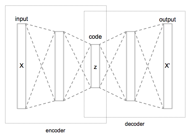
Step 5. 使用 Embedding 層,將「數字 list」轉換為「向量list」

​ Word Embedding 是一種自然語言處理技術,原理是將文字映射成多維幾何空間的向量。類似語意的文字的向量,在多維幾何空間中的距離也比較近。影評文字轉換為數字 list後,數字沒有語意關聯,為了得到關聯性,要轉換為向量。語意相近的詞語,向量會比較接近。

ex:

pleasure -> 38 -> (1.2, 2.3, 3.2)
dislike -> 21 -> (-1.21, 2.7, 3.2)
like -> 10 -> (1.25, 2.33, 3.4)
hate -> 28 -> (-1.5, 2.63, 3.22)

Step 6. 將「向量 list」送入深度學習模型

資料預處理

# get imdb data
import urllib.request
import os
import tarfile

# 下載資料集
import os
if not os.path.exists('data'):
    os.makedirs('data')

url="http://ai.stanford.edu/~amaas/data/sentiment/aclImdb_v1.tar.gz"
filepath="data/aclImdb_v1.tar.gz"
if not os.path.isfile(filepath):
    result=urllib.request.urlretrieve(url,filepath)
    print('downloaded:',result)

if not os.path.exists("data/aclImdb"):
    tfile = tarfile.open("data/aclImdb_v1.tar.gz", 'r:gz')
    result=tfile.extractall('data/')


from keras.datasets import imdb
from keras.preprocessing import sequence
from keras.preprocessing.text import Tokenizer

## rm_tags 可移除文字中的 html tag
import re
def rm_tags(text):
    re_tag = re.compile(r'<[^>]+>')
    return re_tag.sub('', text)

# filetype 為 train 或 test
import os
def read_files(filetype):
    path = "data/aclImdb/"
    file_list=[]

    # 取得檔案 list
    positive_path=path + filetype+"/pos/"
    for f in os.listdir(positive_path):
        file_list+=[positive_path+f]

    negative_path=path + filetype+"/neg/"
    for f in os.listdir(negative_path):
        file_list+=[negative_path+f]

    print('read',filetype, 'files:',len(file_list))

    # 產生 labels,前面 12500 筆為 1,後面 12500 筆為 0
    all_labels = ([1] * 12500 + [0] * 12500)

    # 讀取檔案內容,並去掉 html tag
    all_texts  = []
    for fi in file_list:
        with open(fi,encoding='utf8') as file_input:
            all_texts += [rm_tags(" ".join(file_input.readlines()))]

    return all_labels,all_texts

y_train,train_text=read_files("train")
y_test,test_text=read_files("test")

# #查看正面評價的影評
# print()
# print("train_text[0]=",train_text[0], ", y_train[0]=", y_train[0])

# #查看負面評價的影評
# print("train_text[12500]=", train_text[12500], ", y_train[12500]=", y_train[12500])

###
# 建立 token
# 先讀取所有文章建立字典,限制字典的數量為 nb_words=2000
token = Tokenizer(num_words=2000)
token.fit_on_texts(train_text)

print()
print("token.document_count=", token.document_count)
## token.document_count= 25000
# print("token.word_index=", token.word_index)

# 將每一篇文章的文字轉換一連串的數字
# 只有在字典中的文字會轉換為數字
x_train_seq = token.texts_to_sequences(train_text)
x_test_seq  = token.texts_to_sequences(test_text)

print()
print(train_text[0])
print(x_train_seq[0])

# 讓轉換後的數字長度相同
#文章內的文字,轉換為數字後,每一篇的文章地所產生的數字長度都不同,因為後需要進行類神經網路的訓練,所以每一篇文章所產生的數字長度必須相同
#以下列程式碼為例maxlen=100,所以每一篇文章轉換為數字都必須為100
#如果文章轉成數字大於0,pad_sequences處理後,會truncate前面的數字
x_train = sequence.pad_sequences(x_train_seq, maxlen=100)
x_test  = sequence.pad_sequences(x_test_seq,  maxlen=100)

print()
print('before pad_sequences length=',len(x_train_seq[0]))
print(x_train_seq[0])
print('after pad_sequences length=',len(x_train[0]))
print(x_train[0])

print()
print('before pad_sequences length=',len(x_train_seq[1]))
print(x_train_seq[1])
print('after pad_sequences length=',len(x_train[1]))
print(x_train[1])

####
## 資料預處理

# token = Tokenizer(num_words=2000)
# token.fit_on_texts(train_text)

# x_train_seq = token.texts_to_sequences(train_text)
# x_test_seq  = token.texts_to_sequences(test_text)

# x_train = sequence.pad_sequences(x_train_seq, maxlen=100)
# x_test  = sequence.pad_sequences(x_test_seq,  maxlen=100)

以 MLP 進行情感分析

Model: "sequential_1"
_________________________________________________________________
Layer (type)                 Output Shape              Param #
=================================================================
embedding_1 (Embedding)      (None, 100, 32)           64000
_________________________________________________________________
dropout_1 (Dropout)          (None, 100, 32)           0
_________________________________________________________________
flatten_1 (Flatten)          (None, 3200)              0
_________________________________________________________________
dense_1 (Dense)              (None, 256)               819456
_________________________________________________________________
dropout_2 (Dropout)          (None, 256)               0
_________________________________________________________________
dense_2 (Dense)              (None, 1)                 257
=================================================================
Total params: 883,713
Trainable params: 883,713
Non-trainable params: 0
# get imdb data
import urllib.request
import os
import tarfile

# 下載資料集
import os
if not os.path.exists('data'):
    os.makedirs('data')

url="http://ai.stanford.edu/~amaas/data/sentiment/aclImdb_v1.tar.gz"
filepath="data/aclImdb_v1.tar.gz"
if not os.path.isfile(filepath):
    result=urllib.request.urlretrieve(url,filepath)
    print('downloaded:',result)

if not os.path.exists("data/aclImdb"):
    tfile = tarfile.open("data/aclImdb_v1.tar.gz", 'r:gz')
    result=tfile.extractall('data/')


from keras.datasets import imdb
from keras.preprocessing import sequence
from keras.preprocessing.text import Tokenizer

## rm_tags 可移除文字中的 html tag
import re
def rm_tags(text):
    re_tag = re.compile(r'<[^>]+>')
    return re_tag.sub('', text)

# filetype 為 train 或 test
import os
def read_files(filetype):
    path = "data/aclImdb/"
    file_list=[]

    # 取得檔案 list
    positive_path=path + filetype+"/pos/"
    for f in os.listdir(positive_path):
        file_list+=[positive_path+f]

    negative_path=path + filetype+"/neg/"
    for f in os.listdir(negative_path):
        file_list+=[negative_path+f]

    print('read',filetype, 'files:',len(file_list))

    # 產生 labels,前面 12500 筆為 1,後面 12500 筆為 0
    all_labels = ([1] * 12500 + [0] * 12500)

    # 讀取檔案內容,並去掉 html tag
    all_texts  = []
    for fi in file_list:
        with open(fi,encoding='utf8') as file_input:
            all_texts += [rm_tags(" ".join(file_input.readlines()))]

    return all_labels,all_texts

y_train,train_text=read_files("train")
y_test,test_text=read_files("test")

####
## 資料預處理

token = Tokenizer(num_words=2000)
token.fit_on_texts(train_text)

# 轉成數字 list
x_train_seq = token.texts_to_sequences(train_text)
x_test_seq  = token.texts_to_sequences(test_text)

# 截長補短
x_train = sequence.pad_sequences(x_train_seq, maxlen=100)
x_test  = sequence.pad_sequences(x_test_seq,  maxlen=100)

## 建立模型

from keras.models import Sequential
from keras.layers.core import Dense, Dropout, Activation,Flatten
from keras.layers.embeddings import Embedding

model = Sequential()

# 將 Embedding 層加入模型
# output_dim=32   讓 數字 list 轉輸出成 32 維向量
# input_dim=2000  輸入字典共 2000 字
# input_length=100  因為每一筆資料有 100 個數字
model.add(Embedding(output_dim=32,
                    input_dim=2000,
                    input_length=100))
# Dropout 可避免 overfitting
model.add(Dropout(0.2))

#### 多層感知模型
# 平坦層
# 因為數字 list 為 100,每一個數字轉成 32 維向量
# 100*32 = 3200 個神經元
model.add(Flatten())

# 隱藏層
# 有 256 個神經元
model.add(Dense(units=256,
                activation='relu' ))
model.add(Dropout(0.2))

## 輸出層 1 個神經元
model.add(Dense(units=1,
                activation='sigmoid' ))

print(model.summary())

### 訓練模型
model.compile(loss='binary_crossentropy',
              optimizer='adam',
              metrics=['accuracy'])

# validation_split=0.2    80% 是訓練資料, 20% 是驗證資料
train_history =model.fit(x_train, y_train,batch_size=100,
                         epochs=10,verbose=2,
                         validation_split=0.2)


####################
## 這兩行可解決 ModuleNotFoundError: No module named '_tkinter'
## ref: https://stackoverflow.com/questions/36327134/matplotlib-error-no-module-named-tkinter
import matplotlib
matplotlib.use('agg')
####
import matplotlib.pyplot as plt
def show_train_history(train_acc,test_acc, filename):
    plt.clf()
    plt.gcf()
    plt.plot(train_history.history[train_acc])
    plt.plot(train_history.history[test_acc])
    plt.title('Train History')
    plt.ylabel('Accuracy')
    plt.xlabel('Epoch')
    plt.legend(['train', 'test'], loc='upper left')
    plt.savefig(filename)


show_train_history('acc','val_acc', 'accuracy.png')
show_train_history('loss','val_loss', 'loss.png')


######
# 評估模型準確率
print()
scores = model.evaluate(x_test, y_test, verbose=1)
print("scores[1]=", scores[1])
## scores[1]= 0.81508

####
# 預測機率
probility=model.predict(x_test)

for p in probility[12500:12510]:
    print(p)

## 預測結果
print()
predict=model.predict_classes(x_test)
predict_classes=predict.reshape(-1)
print( predict_classes[:10] )

## 查看預測結果
SentimentDict={1:'正面的',0:'負面的'}
def display_test_Sentiment(i):
    print()
    print(test_text[i])
    print('標籤label:',SentimentDict[y_test[i]],
          '預測結果:',SentimentDict[predict_classes[i]])

display_test_Sentiment(2)
display_test_Sentiment(12502)

#預測新的影評

def predict_review(input_text):
    input_seq = token.texts_to_sequences([input_text])
    pad_input_seq  = sequence.pad_sequences(input_seq , maxlen=100)
    predict_result=model.predict_classes(pad_input_seq)
    print()
    print(SentimentDict[predict_result[0][0]])

predict_review('''
Oh dear, oh dear, oh dear: where should I start folks. I had low expectations already because I hated each and every single trailer so far, but boy did Disney make a blunder here. I'm sure the film will still make a billion dollars - hey: if Transformers 11 can do it, why not Belle? - but this film kills every subtle beautiful little thing that had made the original special, and it does so already in the very early stages. It's like the dinosaur stampede scene in Jackson's King Kong: only with even worse CGI (and, well, kitchen devices instead of dinos).
The worst sin, though, is that everything (and I mean really EVERYTHING) looks fake. What's the point of making a live-action version of a beloved cartoon if you make every prop look like a prop? I know it's a fairy tale for kids, but even Belle's village looks like it had only recently been put there by a subpar production designer trying to copy the images from the cartoon. There is not a hint of authenticity here. Unlike in Jungle Book, where we got great looking CGI, this really is the by-the-numbers version and corporate filmmaking at its worst. Of course it's not really a "bad" film; those 200 million blockbusters rarely are (this isn't 'The Room' after all), but it's so infuriatingly generic and dull - and it didn't have to be. In the hands of a great director the potential for this film would have been huge.
Oh and one more thing: bad CGI wolves (who actually look even worse than the ones in Twilight) is one thing, and the kids probably won't care. But making one of the two lead characters - Beast - look equally bad is simply unforgivably stupid. No wonder Emma Watson seems to phone it in: she apparently had to act against an guy with a green-screen in the place where his face should have been.
''')

predict_review('''
It's hard to believe that the same talented director who made the influential cult action classic The Road Warrior had anything to do with this disaster.
Road Warrior was raw, gritty, violent and uncompromising, and this movie is the exact opposite. It's like Road Warrior for kids who need constant action in their movies.
This is the movie. The good guys get into a fight with the bad guys, outrun them, they break down in their vehicle and fix it. Rinse and repeat. The second half of the movie is the first half again just done faster.
The Road Warrior may have been a simple premise but it made you feel something, even with it's opening narration before any action was even shown. And the supporting characters were given just enough time for each of them to be likable or relatable.
In this movie there is absolutely nothing and no one to care about. We're supposed to care about the characters because... well we should. George Miller just wants us to, and in one of the most cringe worthy moments Charlize Theron's character breaks down while dramatic music plays to try desperately to make us care.
Tom Hardy is pathetic as Max. One of the dullest leading men I've seen in a long time. There's not one single moment throughout the entire movie where he comes anywhere near reaching the same level of charisma Mel Gibson did in the role. Gibson made more of an impression just eating a tin of dog food. I'm still confused as to what accent Hardy was even trying to do.
I was amazed that Max has now become a cartoon character as well. Gibson's Max was a semi-realistic tough guy who hurt, bled, and nearly died several times. Now he survives car crashes and tornadoes with ease?
In the previous movies, fuel and guns and bullets were rare. Not anymore. It doesn't even seem Post-Apocalyptic. There's no sense of desperation anymore and everything is too glossy looking. And the main villain's super model looking wives with their perfect skin are about as convincing as apocalyptic survivors as Hardy's Australian accent is. They're so boring and one-dimensional, George Miller could have combined them all into one character and you wouldn't miss anyone.
Some of the green screen is very obvious and fake looking, and the CGI sandstorm is laughably bad. It wouldn't look out of place in a Pixar movie.
There's no tension, no real struggle, or any real dirt and grit that Road Warrior had. Everything George Miller got right with that masterpiece he gets completely wrong here.
''')

# serialize model to JSON

if not os.path.exists('SaveModel'):
    os.makedirs('SaveModel')

model_json = model.to_json()
with open("SaveModel/Imdb_RNN_model.json", "w") as json_file:
    json_file.write(model_json)

model.save_weights("SaveModel/Imdb_RNN_model.h5")
print("Saved model to disk")

用較大的字典數量,改善準確率 由 scores[1]= 0.81508 改善為 scores[1]= 0.85388

字典數量 3800

數字 list 長度為 380

遞迴神經網路 RNN

自然語言處理的問題中,資料具有順序性,因為 MLP, CNN 都只能依照目前的狀態進行辨識,如果要處理有時間序列的問題,必須改用 RNN, LSTM 模型

RNN 的神經元具有記憶的功能

在 t 時間點

  • \(X_t\) 是 t 時間點神經網路的輸入

  • \(O_t\) 是 t 時間點神經網路的輸出

  • (U, V, W) 是神經網路的參數, W 參數是 t-1 時間點的輸出,作為 t 時間點的輸入

  • \(S_t\) 是隱藏狀態,代表神經網路的記憶,經過目前時間點的輸入 \(X_t\) 再加上上一個時間點的狀態 \(S_{t-1}\) ,再加上 U, W 參數的評估結果

    \(S_t = f([U]X_t+[W]S_{t-1})\) 其中 f 為非線性函數,例如 ReLU

RNN 流程

keras_imdb_6.jpg

Model: "sequential_1"
_________________________________________________________________
Layer (type)                 Output Shape              Param #
=================================================================
embedding_1 (Embedding)      (None, 380, 32)           121600
_________________________________________________________________
dropout_1 (Dropout)          (None, 380, 32)           0
_________________________________________________________________
simple_rnn_1 (SimpleRNN)     (None, 16)                784
_________________________________________________________________
dense_1 (Dense)              (None, 256)               4352
_________________________________________________________________
dropout_2 (Dropout)          (None, 256)               0
_________________________________________________________________
dense_2 (Dense)              (None, 1)                 257
=================================================================
Total params: 126,993
Trainable params: 126,993
Non-trainable params: 0
# get imdb data
import urllib.request
import os
import tarfile

# 下載資料集
import os
if not os.path.exists('data'):
    os.makedirs('data')

url="http://ai.stanford.edu/~amaas/data/sentiment/aclImdb_v1.tar.gz"
filepath="data/aclImdb_v1.tar.gz"
if not os.path.isfile(filepath):
    result=urllib.request.urlretrieve(url,filepath)
    print('downloaded:',result)

if not os.path.exists("data/aclImdb"):
    tfile = tarfile.open("data/aclImdb_v1.tar.gz", 'r:gz')
    result=tfile.extractall('data/')


from keras.datasets import imdb
from keras.preprocessing import sequence
from keras.preprocessing.text import Tokenizer

## rm_tags 可移除文字中的 html tag
import re
def rm_tags(text):
    re_tag = re.compile(r'<[^>]+>')
    return re_tag.sub('', text)

# filetype 為 train 或 test
import os
def read_files(filetype):
    path = "data/aclImdb/"
    file_list=[]

    # 取得檔案 list
    positive_path=path + filetype+"/pos/"
    for f in os.listdir(positive_path):
        file_list+=[positive_path+f]

    negative_path=path + filetype+"/neg/"
    for f in os.listdir(negative_path):
        file_list+=[negative_path+f]

    print('read',filetype, 'files:',len(file_list))

    # 產生 labels,前面 12500 筆為 1,後面 12500 筆為 0
    all_labels = ([1] * 12500 + [0] * 12500)

    # 讀取檔案內容,並去掉 html tag
    all_texts  = []
    for fi in file_list:
        with open(fi,encoding='utf8') as file_input:
            all_texts += [rm_tags(" ".join(file_input.readlines()))]

    return all_labels,all_texts

y_train,train_text=read_files("train")
y_test,test_text=read_files("test")

####
## 資料預處理

token = Tokenizer(num_words=3800)
token.fit_on_texts(train_text)

# 轉成數字 list
x_train_seq = token.texts_to_sequences(train_text)
x_test_seq  = token.texts_to_sequences(test_text)

# 截長補短
x_train = sequence.pad_sequences(x_train_seq, maxlen=380)
x_test  = sequence.pad_sequences(x_test_seq,  maxlen=380)

## 建立模型

from keras.models import Sequential
from keras.layers.core import Dense, Dropout, Activation
from keras.layers.embeddings import Embedding
from keras.layers.recurrent import SimpleRNN

model = Sequential()

# 將 Embedding 層加入模型
# output_dim=32   讓 數字 list 轉輸出成 32 維向量
# input_dim=3800  輸入字典共 3800 字
# input_length=100  因為每一筆資料有 100 個數字
model.add(Embedding(output_dim=32,
                    input_dim=3800,
                    input_length=380))
# Dropout 可避免 overfitting
model.add(Dropout(0.2))

#### RNN
model.add(SimpleRNN(units=32))

model.add(Dense(units=256,activation='relu' ))
model.add(Dropout(0.2))

model.add(Dense(units=1,activation='sigmoid' ))

print(model.summary())

### 訓練模型
model.compile(loss='binary_crossentropy',
              optimizer='adam',
              metrics=['accuracy'])

# validation_split=0.2    80% 是訓練資料, 20% 是驗證資料
train_history =model.fit(x_train, y_train,batch_size=100,
                         epochs=10,verbose=2,
                         validation_split=0.2)


####################
## 這兩行可解決 ModuleNotFoundError: No module named '_tkinter'
## ref: https://stackoverflow.com/questions/36327134/matplotlib-error-no-module-named-tkinter
import matplotlib
matplotlib.use('agg')
####
import matplotlib.pyplot as plt
def show_train_history(train_acc,test_acc, filename):
    plt.clf()
    plt.gcf()
    plt.plot(train_history.history[train_acc])
    plt.plot(train_history.history[test_acc])
    plt.title('Train History')
    plt.ylabel('Accuracy')
    plt.xlabel('Epoch')
    plt.legend(['train', 'test'], loc='upper left')
    plt.savefig(filename)


show_train_history('acc','val_acc', 'accuracy.png')
show_train_history('loss','val_loss', 'loss.png')


######
# 評估模型準確率
print()
scores = model.evaluate(x_test, y_test, verbose=1)
print("scores[1]=", scores[1])
## scores[1]= 0.83972

####
# 預測機率
probility=model.predict(x_test)

for p in probility[12500:12510]:
    print(p)

## 預測結果
print()
predict=model.predict_classes(x_test)
predict_classes=predict.reshape(-1)
print( predict_classes[:10] )

## 查看預測結果
SentimentDict={1:'正面的',0:'負面的'}
def display_test_Sentiment(i):
    print()
    print(test_text[i])
    print('標籤label:',SentimentDict[y_test[i]],
          '預測結果:',SentimentDict[predict_classes[i]])

display_test_Sentiment(2)
display_test_Sentiment(12502)

#預測新的影評

def predict_review(input_text):
    input_seq = token.texts_to_sequences([input_text])
    pad_input_seq  = sequence.pad_sequences(input_seq , maxlen=380)
    predict_result=model.predict_classes(pad_input_seq)
    print()
    print(SentimentDict[predict_result[0][0]])

predict_review('''
Oh dear, oh dear, oh dear: where should I start folks. I had low expectations already because I hated each and every single trailer so far, but boy did Disney make a blunder here. I'm sure the film will still make a billion dollars - hey: if Transformers 11 can do it, why not Belle? - but this film kills every subtle beautiful little thing that had made the original special, and it does so already in the very early stages. It's like the dinosaur stampede scene in Jackson's King Kong: only with even worse CGI (and, well, kitchen devices instead of dinos).
The worst sin, though, is that everything (and I mean really EVERYTHING) looks fake. What's the point of making a live-action version of a beloved cartoon if you make every prop look like a prop? I know it's a fairy tale for kids, but even Belle's village looks like it had only recently been put there by a subpar production designer trying to copy the images from the cartoon. There is not a hint of authenticity here. Unlike in Jungle Book, where we got great looking CGI, this really is the by-the-numbers version and corporate filmmaking at its worst. Of course it's not really a "bad" film; those 200 million blockbusters rarely are (this isn't 'The Room' after all), but it's so infuriatingly generic and dull - and it didn't have to be. In the hands of a great director the potential for this film would have been huge.
Oh and one more thing: bad CGI wolves (who actually look even worse than the ones in Twilight) is one thing, and the kids probably won't care. But making one of the two lead characters - Beast - look equally bad is simply unforgivably stupid. No wonder Emma Watson seems to phone it in: she apparently had to act against an guy with a green-screen in the place where his face should have been.
''')

predict_review('''
It's hard to believe that the same talented director who made the influential cult action classic The Road Warrior had anything to do with this disaster.
Road Warrior was raw, gritty, violent and uncompromising, and this movie is the exact opposite. It's like Road Warrior for kids who need constant action in their movies.
This is the movie. The good guys get into a fight with the bad guys, outrun them, they break down in their vehicle and fix it. Rinse and repeat. The second half of the movie is the first half again just done faster.
The Road Warrior may have been a simple premise but it made you feel something, even with it's opening narration before any action was even shown. And the supporting characters were given just enough time for each of them to be likable or relatable.
In this movie there is absolutely nothing and no one to care about. We're supposed to care about the characters because... well we should. George Miller just wants us to, and in one of the most cringe worthy moments Charlize Theron's character breaks down while dramatic music plays to try desperately to make us care.
Tom Hardy is pathetic as Max. One of the dullest leading men I've seen in a long time. There's not one single moment throughout the entire movie where he comes anywhere near reaching the same level of charisma Mel Gibson did in the role. Gibson made more of an impression just eating a tin of dog food. I'm still confused as to what accent Hardy was even trying to do.
I was amazed that Max has now become a cartoon character as well. Gibson's Max was a semi-realistic tough guy who hurt, bled, and nearly died several times. Now he survives car crashes and tornadoes with ease?
In the previous movies, fuel and guns and bullets were rare. Not anymore. It doesn't even seem Post-Apocalyptic. There's no sense of desperation anymore and everything is too glossy looking. And the main villain's super model looking wives with their perfect skin are about as convincing as apocalyptic survivors as Hardy's Australian accent is. They're so boring and one-dimensional, George Miller could have combined them all into one character and you wouldn't miss anyone.
Some of the green screen is very obvious and fake looking, and the CGI sandstorm is laughably bad. It wouldn't look out of place in a Pixar movie.
There's no tension, no real struggle, or any real dirt and grit that Road Warrior had. Everything George Miller got right with that masterpiece he gets completely wrong here.
''')

# serialize model to JSON

if not os.path.exists('SaveModel'):
    os.makedirs('SaveModel')

model_json = model.to_json()
with open("SaveModel/Imdb_RNN_model.json", "w") as json_file:
    json_file.write(model_json)

model.save_weights("SaveModel/Imdb_RNN_model.h5")
print("Saved model to disk")

LSTM 模型

RNN 在訓練時,會發生 long-term dependencies 的問題,這是因為 RNN 會遇到梯度消失或爆炸 vanishing/exploding 的問題,訓練時在計算與反向傳播,梯度傾向於在每一個時刻遞增或遞減,經過一段時間後,會發散到無限大或收斂到 0

long-term dependencies 的問題,就是在每一個時間的間隔不斷增加時, RNN 會失去學習到連接遠的訊息的能力。如下圖: 隨著時間點 t 不段遞增,到了後期 t,隱藏狀態 \(S_t\) 已經失去學習 \(X_0\) 的能力。導致神經網路不能知道,我是在台北市市政府上班。

RNN 只能取得短期記憶,不記得長期記憶,因此有 LSTM 模型解決此問題

LSTM 中,一個神經元相當於一個記憶細胞 cell

  • \(X_t\) 輸入向量
  • \(Y_t\) 輸出向量
  • \(C_t\): cell ,是 LSTM 的記憶細胞狀態 cell state
  • LSTM 利用 gate 機制,控制記憶細胞狀態,刪減或增加裡面的訊息
    • \(I_t\) Input Gate 用來決定哪些訊息要增加到 cell
    • \(F_t\) Forget Gate 決定哪些訊息要被刪減
    • \(O_t\) Output Gate 決定要從 cell 輸出哪些訊息

有了 Gate, LSTM 就能記住長期記憶

程式只需要修改 model

model = Sequential()

# 將 Embedding 層加入模型
# output_dim=32   讓 數字 list 轉輸出成 32 維向量
# input_dim=3800  輸入字典共 3800 字
# input_length=100  因為每一筆資料有 100 個數字
model.add(Embedding(output_dim=32,
                    input_dim=3800,
                    input_length=380))
# Dropout 可避免 overfitting
model.add(Dropout(0.2))

#### LSTM
model.add( LSTM(32) )

model.add(Dense(units=256,activation='relu' ))
model.add(Dropout(0.2))

model.add(Dense(units=1,activation='sigmoid' ))

評估模型準確率:

  1. MLP 100

    scores[1]= 0.81508

  2. MLP 380

    scores[1]= 0.84252

  3. RNN

    scores[1]= 0.83972

  4. LSTM

    scores[1]= 0.85792

References

TensorFlow+Keras深度學習人工智慧實務應用

2020/09/21

keras手寫數字辨識_AutoEncoder

MNIST AutoEncoder

Autoencoder是一種可以將資料中的重要資訊保留下來的神經網路,有點像是資料壓縮,在做資料壓縮時,會有一個 Encoder 可以壓縮資料,另外還有一個 Decoder,可以還原資料。壓縮的過程就是用更精簡的方式保存了資料。Autoencoder 跟一般資料壓縮類似,也有 Encoder和Decoder,但 Decoder 的結果,不能確保可以完全還原。

Autoencoder會試著從測試資料,自己學習出Encoder和Decoder,並盡量讓資料在壓縮後又可以還原回去。實際上最常見的應用是,對圖片進行降噪 DeNoise。Autoencoder 是一種資料壓縮/解壓縮演算法,能夠處理 (1) 特定資料 (2) 壓縮後會遺失部分資訊,也就是無法完整還原回原本的資料 (3) 可由訓練資料中自動學習壓縮的方法。特定資料的意思跟常見的語音壓縮 mp3 不同,MPEG-2 Audio Layer III (mp3),可以處理所有的語音資料,但 AutoEncoder 訓練的結果,只能處理跟訓練資料類似的語音資料。例如處理人臉圖片的 autoencoder,無法有效處理 tree 的圖片。

不管是「Encoder」還是「Decoder」都可以調整權重,如果將Encoder+Decoder的結構建立好並搭配Input當作Output的目標答案,在訓練的過程中,Autoencoder會試著找出最好的權重來使得資訊可以盡量完整還原回去,換句話說,Autoencoder可以自行找出了Encoder和Decoder。

Encoder 的效果等同於做 Dimension Reduction,Encoder會轉換原本的資料到一個新的空間,這個空間可以比原本Features描述的空間更能精簡的描述這群數據,而中間這層Layer的數值Embedding Code就是新空間裡頭的座標,有些時候我們會用這個新空間來判斷每筆資料之間的接近程度。

理論上是無法做出一個 autoencoder,其得到的壓縮效果,能夠跟類似 jpeg, mp3 這種壓縮方法一樣好,因為我們無法取得「所有」的語音/圖片資料,進行訓練。

目前 autoencoder 有兩個實用的應用:(1) data denoising 例如圖片降噪 (2) dimensionality reduction for data visulization 對於多維度離散的資料,autoencoder 能夠學習出 data projection,功能跟 PCA (Principla Compoenent Analysis) 或 t-SNE 一樣,但效果更好。(ref: 淺談降維方法中的 PCA 與 t-SNE

Simple Autoencoder

# -*- coding: utf-8 -*-
from keras.datasets import mnist
from keras.utils import np_utils
import numpy as np
np.random.seed(10)

# 讀取 mnist 資料
(x_train, y_train), (x_test, y_test) = mnist.load_data()

# 標準化
x_train = x_train.astype('float32') / 255.
x_test = x_test.astype('float32') / 255.

# 正規化資料維度,以便 Keras 處理
x_train = x_train.reshape((len(x_train), np.prod(x_train.shape[1:])))
x_test = x_test.reshape((len(x_test), np.prod(x_test.shape[1:])))

print("x_train.shape=",x_train.shape, ", x_test.shape=",x_test.shape)

# simple autoencoder
# 建立 Autoencoder Model 並使用 x_train 資料進行訓練
from keras.layers import Input, Dense
from keras.models import Model

# this is the size of our encoded representations
encoding_dim = 32  # 32 floats -> compression of factor 24.5, assuming the input is 784 floats

# this is our input placeholder
input_img = Input(shape=(784,))
# "encoded" is the encoded representation of the input
encoded = Dense(encoding_dim, activation='relu')(input_img)
# "decoded" is the lossy reconstruction of the input
decoded = Dense(784, activation='sigmoid')(encoded)

# 建立 Model 並將 loss funciton 設為 binary cross entropy
# this model maps an input to its reconstruction
autoencoder = Model(input_img, decoded)
autoencoder.compile(optimizer='adadelta', loss='binary_crossentropy')

autoencoder.fit(x_train,
                x_train,  # Label 也設為 x_train
                epochs=25,
                batch_size=128,
                shuffle=True,
                validation_data=(x_test, x_test))

##########
# 另外製作 encoder, decoder 兩個分開的 Model
# this model maps an input to its encoded representation
encoder = Model(input_img, encoded)

# create a placeholder for an encoded (32-dimensional) input
encoded_input = Input(shape=(encoding_dim,))
# retrieve the last layer of the autoencoder model
decoder_layer = autoencoder.layers[-1]
# create the decoder model
decoder = Model(encoded_input, decoder_layer(encoded_input))

# encode and decode some digits
# note that we take them from the *test* set
encoded_imgs = encoder.predict(x_test)
decoded_imgs = decoder.predict(encoded_imgs)

# use Matplotlib
import matplotlib
matplotlib.use('agg')

import matplotlib.pyplot as plt
plt.clf()
n = 10  # how many digits we will display
plt.figure(figsize=(20, 4))
for i in range(n):
    # display original
    ax = plt.subplot(2, n, i + 1)
    plt.imshow(x_test[i].reshape(28, 28))
    plt.gray()
    ax.get_xaxis().set_visible(False)
    ax.get_yaxis().set_visible(False)

    # display reconstruction
    ax = plt.subplot(2, n, i + 1 + n)
    plt.imshow(decoded_imgs[i].reshape(28, 28))
    plt.gray()
    ax.get_xaxis().set_visible(False)
    ax.get_yaxis().set_visible(False)
plt.savefig("auto.png")

訓練過程

60000/60000 [==============================] - 4s 62us/step - loss: 0.3079 - val_loss: 0.2502
Epoch 2/25
60000/60000 [==============================] - 1s 12us/step - loss: 0.2300 - val_loss: 0.2105
Epoch 3/25
60000/60000 [==============================] - 1s 12us/step - loss: 0.2009 - val_loss: 0.1898
Epoch 4/25
60000/60000 [==============================] - 1s 13us/step - loss: 0.1839 - val_loss: 0.1756
Epoch 5/25
60000/60000 [==============================] - 1s 14us/step - loss: 0.1715 - val_loss: 0.1650
Epoch 6/25
60000/60000 [==============================] - 1s 13us/step - loss: 0.1619 - val_loss: 0.1563
Epoch 7/25
60000/60000 [==============================] - 1s 12us/step - loss: 0.1540 - val_loss: 0.1490
Epoch 8/25
60000/60000 [==============================] - 1s 12us/step - loss: 0.1473 - val_loss: 0.1429
Epoch 9/25
60000/60000 [==============================] - 1s 12us/step - loss: 0.1415 - val_loss: 0.1373
Epoch 10/25
60000/60000 [==============================] - 1s 12us/step - loss: 0.1365 - val_loss: 0.1325
Epoch 11/25
60000/60000 [==============================] - 1s 12us/step - loss: 0.1320 - val_loss: 0.1282
Epoch 12/25
60000/60000 [==============================] - 1s 12us/step - loss: 0.1279 - val_loss: 0.1243
Epoch 13/25
60000/60000 [==============================] - 1s 12us/step - loss: 0.1242 - val_loss: 0.1208
Epoch 14/25
60000/60000 [==============================] - 1s 12us/step - loss: 0.1209 - val_loss: 0.1178
Epoch 15/25
60000/60000 [==============================] - 1s 12us/step - loss: 0.1180 - val_loss: 0.1151
Epoch 16/25
60000/60000 [==============================] - 1s 12us/step - loss: 0.1155 - val_loss: 0.1127
Epoch 17/25
60000/60000 [==============================] - 1s 12us/step - loss: 0.1133 - val_loss: 0.1107
Epoch 18/25
60000/60000 [==============================] - 1s 12us/step - loss: 0.1115 - val_loss: 0.1090
Epoch 19/25
60000/60000 [==============================] - 1s 12us/step - loss: 0.1098 - val_loss: 0.1075
Epoch 20/25
60000/60000 [==============================] - 1s 12us/step - loss: 0.1085 - val_loss: 0.1062
Epoch 21/25
60000/60000 [==============================] - 1s 12us/step - loss: 0.1073 - val_loss: 0.1051
Epoch 22/25
60000/60000 [==============================] - 1s 14us/step - loss: 0.1062 - val_loss: 0.1042
Epoch 23/25
60000/60000 [==============================] - 1s 13us/step - loss: 0.1053 - val_loss: 0.1033
Epoch 24/25
60000/60000 [==============================] - 1s 15us/step - loss: 0.1046 - val_loss: 0.1026
Epoch 25/25
60000/60000 [==============================] - 1s 12us/step - loss: 0.1039 - val_loss: 0.1020

這是測試的前10 筆資料,上面是原始測試圖片,下面是經過壓縮/解壓縮後,產生的圖片,因為是簡單的 autoencoder,目前的效果還不夠好。

Sparse Autoencoder

ref: Tensorflow Day17 Sparse Autoencoder

在 encoded representation 加上 sparsity constraint

原本只有限制 hidden layer 為 32 維,在 hidden representation 加上 sparsity constraint。原本所有神經元會對所有輸入資料都有反應,但我們希望神經元只對某一些訓練資料有反應,例如神經元 A 對 5 有反應,B 只對 7 有反應。讓神經元有對每一個數字都有專業工作。

可在 loss function 加上兩項,達到這個限制

  • Sparsity Regularization
  • L2 Regularization

將 activity_regularizer 增加到 Dense Layer,並將訓練次數改為 100 次(因為增加了constraint,可以訓練更多次,而不會發生 overfitting)

# this is our input placeholder
input_img = Input(shape=(784,))
# "encoded" is the encoded representation of the input
# add a Dense layer with a L1 activity regularizer
encoded = Dense(encoding_dim, activation='relu',
                activity_regularizer=regularizers.l1(10e-5))(input_img)

# "decoded" is the lossy reconstruction of the input
decoded = Dense(784, activation='sigmoid')(encoded)

Note: 實際上這個部分測試的結果,反而變更差,目前不知道原因

Epoch 100/100
60000/60000 [==============================] - 1s 12us/step - loss: 0.2612 - val_loss: 0.2603

Deep AutoEncoder

在 encoded, decoded 從原本的一層,改為 3 層

# -*- coding: utf-8 -*-
from keras.datasets import mnist
from keras.utils import np_utils
import numpy as np
np.random.seed(10)

# 讀取 mnist 資料
(x_train, y_train), (x_test, y_test) = mnist.load_data()

# 標準化
x_train = x_train.astype('float32') / 255.
x_test = x_test.astype('float32') / 255.

# 正規化資料維度,以便 Keras 處理
x_train = x_train.reshape((len(x_train), np.prod(x_train.shape[1:])))
x_test = x_test.reshape((len(x_test), np.prod(x_test.shape[1:])))

print("x_train.shape=",x_train.shape, ", x_test.shape=",x_test.shape)

# simple autoencoder
# 建立 Autoencoder Model 並使用 x_train 資料進行訓練
from keras.layers import Input, Dense
from keras.models import Model
from keras import regularizers

# this is the size of our encoded representations
encoding_dim = 32  # 32 floats -> compression of factor 24.5, assuming the input is 784 floats

input_img = Input(shape=(784,))
encoded = Dense(128, activation='relu')(input_img)
encoded = Dense(64, activation='relu')(encoded)
encoded = Dense(32, activation='relu')(encoded)

decoded = Dense(64, activation='relu')(encoded)
decoded = Dense(128, activation='relu')(decoded)
decoded = Dense(784, activation='sigmoid')(decoded)

# 建立 Model 並將 loss funciton 設為 binary cross entropy
# this model maps an input to its reconstruction
autoencoder = Model(input_img, decoded)
autoencoder.compile(optimizer='adadelta', loss='binary_crossentropy')

autoencoder.fit(x_train,
                x_train,  # Label 也設為 x_train
                epochs=100,
                batch_size=128,
                shuffle=True,
                validation_data=(x_test, x_test))


# _________________________________________________________________
# Layer (type)                 Output Shape              Param #
# =================================================================
# input_1 (InputLayer)         (None, 784)               0
# _________________________________________________________________
# dense_1 (Dense)              (None, 128)               100480
# _________________________________________________________________
# dense_2 (Dense)              (None, 64)                8256
# _________________________________________________________________
# dense_3 (Dense)              (None, 32)                2080
# _________________________________________________________________
# dense_4 (Dense)              (None, 64)                2112
# _________________________________________________________________
# dense_5 (Dense)              (None, 128)               8320
# _________________________________________________________________
# dense_6 (Dense)              (None, 784)               101136
# =================================================================
# Total params: 222,384
# Trainable params: 222,384
# Non-trainable params: 0

decoded_imgs = autoencoder.predict(x_test)

# use Matplotlib
import matplotlib
matplotlib.use('agg')

import matplotlib.pyplot as plt
plt.clf()
n = 10  # how many digits we will display
plt.figure(figsize=(20, 4))
for i in range(n):
    # display original
    ax = plt.subplot(2, n, i + 1)
    plt.imshow(x_test[i].reshape(28, 28))
    plt.gray()
    ax.get_xaxis().set_visible(False)
    ax.get_yaxis().set_visible(False)

    # display reconstruction
    ax = plt.subplot(2, n, i + 1 + n)
    plt.imshow(decoded_imgs[i].reshape(28, 28))
    plt.gray()
    ax.get_xaxis().set_visible(False)
    ax.get_yaxis().set_visible(False)
plt.savefig("auto.png")

訓練結果 loss rate 由 0.1 降到 0.09

Epoch 100/100
60000/60000 [==============================] - 2s 33us/step - loss: 0.0927 - val_loss: 0.0925

Convolutional Autoencoder

執行前要加上環境變數

export TF_FORCE_GPU_ALLOW_GROWTH=true

執行結果

Epoch 50/50
60000/60000 [==============================] - 3s 57us/step - loss: 0.1012 - val_loss: 0.0984

Image Denoise

用加上 noise 的圖片當作 input,output 為沒有 noise 的圖片,這樣進行 model 訓練

# -*- coding: utf-8 -*-
from keras.datasets import mnist
from keras.utils import np_utils
import numpy as np
np.random.seed(10)

# 讀取 mnist 資料
(x_train, y_train), (x_test, y_test) = mnist.load_data()

# 標準化
x_train = x_train.astype('float32') / 255.
x_test = x_test.astype('float32') / 255.

# 正規化資料維度,以便 Keras 處理
x_train = np.reshape(x_train, (len(x_train), 28, 28, 1))  # adapt this if using `channels_first` image data format
x_test = np.reshape(x_test, (len(x_test), 28, 28, 1))  # adapt this if using `channels_first` image data format


# 將原圖加上 noise
noise_factor = 0.5
x_train_noisy = x_train + noise_factor * np.random.normal(loc=0.0, scale=1.0, size=x_train.shape)
x_test_noisy = x_test + noise_factor * np.random.normal(loc=0.0, scale=1.0, size=x_test.shape)

x_train_noisy = np.clip(x_train_noisy, 0., 1.)
x_test_noisy = np.clip(x_test_noisy, 0., 1.)


print("x_train.shape=",x_train.shape, ", x_test.shape=",x_test.shape)

from keras.layers import Input, Dense, Conv2D, MaxPooling2D, UpSampling2D
from keras.models import Model
from keras import backend as K

input_img = Input(shape=(28, 28, 1))  # adapt this if using `channels_first` image data format

## model

x = Conv2D(32, (3, 3), activation='relu', padding='same')(input_img)
x = MaxPooling2D((2, 2), padding='same')(x)
x = Conv2D(32, (3, 3), activation='relu', padding='same')(x)
encoded = MaxPooling2D((2, 2), padding='same')(x)

# at this point the representation is (7, 7, 32)

x = Conv2D(32, (3, 3), activation='relu', padding='same')(encoded)
x = UpSampling2D((2, 2))(x)
x = Conv2D(32, (3, 3), activation='relu', padding='same')(x)
x = UpSampling2D((2, 2))(x)
decoded = Conv2D(1, (3, 3), activation='sigmoid', padding='same')(x)

autoencoder = Model(input_img, decoded)

autoencoder.compile(optimizer='adadelta', loss='binary_crossentropy')

autoencoder.fit(x_train_noisy,
                x_train,  # Label 也設為 x_train
                epochs=100,
                batch_size=128,
                shuffle=True,
                validation_data=(x_test_noisy, x_test))


decoded_imgs = autoencoder.predict(x_test_noisy)

# use Matplotlib
import matplotlib
matplotlib.use('agg')

import matplotlib.pyplot as plt
plt.clf()
n = 10  # how many digits we will display
plt.figure(figsize=(20, 4))
for i in range(n):
    # display original
    ax = plt.subplot(2, n, i + 1)
    plt.imshow(x_test_noisy[i].reshape(28, 28))
    plt.gray()
    ax.get_xaxis().set_visible(False)
    ax.get_yaxis().set_visible(False)

    # display reconstruction
    ax = plt.subplot(2, n, i + 1 + n)
    plt.imshow(decoded_imgs[i].reshape(28, 28))
    plt.gray()
    ax.get_xaxis().set_visible(False)
    ax.get_yaxis().set_visible(False)
plt.savefig("auto.png")

結果

Epoch 100/100
60000/60000 [==============================] - 3s 56us/step - loss: 0.0941 - val_loss: 0.0941

Sequence-to-sequence Autoencoder

如果輸入的資料是 sequence,而不是 vector / 2D image,如果想要有 temporal structure 的 model 要改用 LSTM

from keras.layers import Input, LSTM, RepeatVector
from keras.models import Model

inputs = Input(shape=(timesteps, input_dim))
encoded = LSTM(latent_dim)(inputs)

decoded = RepeatVector(timesteps)(encoded)
decoded = LSTM(input_dim, return_sequences=True)(decoded)

sequence_autoencoder = Model(inputs, decoded)
encoder = Model(inputs, encoded)

Variational autoencoder (VAE)

variational autoencoder 是在 encoded representation 中增加 constraints 的 autoencoder。也就是 latent variable model,就是要學習一個原始資料統計分佈模型,接下來可用此模型,產生新的資料。

ref: variational_autoencoder.py

References

Building Autoencoders in Keras

Autoencoder 簡介與應用範例

[實戰系列] 使用 Keras 搭建一個 Denoising AE 魔法陣(模型)

機器學習技法 學習筆記 (6):神經網路(Neural Network)與深度學習(Deep Learning)

實作Tensorflow (4):Autoencoder

自編碼 Autoencoder (非監督學習)

[TensorFlow] [Keras] kernelregularizer、biasregularizer 和 activity_regularizer

2020/09/14

TensorFlow張量運算

TensorFlow 跟 Keras 最大的差異是,TensorFlow 必須要自行設計張量(矩陣)運算。

計算圖 Computational Graph

TensorFlow 設計核心是計算圖 Computational Graph,可分兩個部分:建立計算圖,及執行計算圖。

  1. 建立計算圖

    透過 TensorFlow 的模組,建立計算圖。

  2. 執行計算圖

    建立計算圖後,可產生 Session 執行計算圖。Session 的作用是在用戶端與執行裝置之間建立連結,有了連結,就可在不同裝置中,執行計算圖,後續任何跟裝置間的資料傳遞,都必須透過 Session 才能進行。

import tensorflow as tf

# 建立 tensorflow 常數, 常數值為 2, 名稱為 ts_c
ts_c = tf.constant(2,name='ts_c')
# 建立 tensorflow 變數,數值為剛剛的常數 + 5, 名稱為 ts_x
ts_x = tf.Variable(ts_c+5,name='ts_x')
print(ts_c)
## Tensor("ts_c:0", shape=(), dtype=int32)
## Tensor       就是 tensorflow 張量
## shape=()     代表這是 0 維的 tensor,也就是數值
## dtype=int32  張量資料型別為 int32
print(ts_x)
## <tf.Variable 'ts_x:0' shape=() dtype=int32_ref>


#######
# 建立 Session 執行 計算圖

# 產生 session
sess=tf.Session()
# 初始化所有 tensorflow global 變數
init = tf.global_variables_initializer()
sess.run(init)

# 透過 sess.run 執行計算圖,並列印執行結果
print('ts_c=',sess.run(ts_c))
print('ts_x=',sess.run(ts_x))

# 使用 eval,顯示 tensorflow 常數
print('ts_c=',ts_c.eval(session=sess))
print('ts_x=',ts_x.eval(session=sess))

# 不需要再使用 session 時,必須用 close 關閉 session
sess.close()

執行結果

ts_c= 2
ts_x= 7
ts_c= 2
ts_x= 7

可改用 With 語法,就不需要寫 sess.close(),會自動關閉,可解決可能沒有關閉 session 的問題,發生的原因,可能是程式忘了寫,或是中途發生錯誤。

import tensorflow as tf

# 建立 tensorflow 常數, 常數值為 2, 名稱為 ts_c
ts_c = tf.constant(2,name='ts_c')
# 建立 tensorflow 變數,數值為剛剛的常數 + 5, 名稱為 ts_x
ts_x = tf.Variable(ts_c+5,name='ts_x')
print(ts_c)
## Tensor("ts_c:0", shape=(), dtype=int32)
## Tensor       就是 tensorflow 張量
## shape=()     代表這是 0 維的 tensor,也就是數值
## dtype=int32  張量資料型別為 int32
print(ts_x)
## <tf.Variable 'ts_x:0' shape=() dtype=int32_ref>


#######
# 建立 Session 執行 計算圖

with tf.Session() as sess:
    # 初始化所有 tensorflow global 變數
    init = tf.global_variables_initializer()
    sess.run(init)

    # 透過 sess.run 執行計算圖,並列印執行結果
    print('ts_c=',sess.run(ts_c))
    print('ts_x=',sess.run(ts_x))

placeholder

剛剛建立計算圖時,常數與變數都是在建立計算圖的階段,就設定好了。但如果我們希望能在執行計算圖的階段,再設定數值,就必須使用 placeholder。

import tensorflow as tf

# 建立兩個 placeholder,然後用 multiply 相乘,結果存入 area
width = tf.placeholder("int32")
height = tf.placeholder("int32")
area=tf.multiply(width,height)

#######
# 建立 Session 執行 計算圖
# 在 sess.run 傳入 feed_dict 參數 {width: 6, height: 8}
with tf.Session() as sess:
    init = tf.global_variables_initializer()
    sess.run(init)
    print('area=',sess.run(area, feed_dict={width: 6, height: 8}))
    # area= 48

deprecated -> 改為tf.compat.v1.

import tensorflow as tf

# 建立兩個 placeholder,然後用 multiply 相乘,結果存入 area
width = tf.compat.v1.placeholder("int32")
height = tf.compat.v1.placeholder("int32")
area=tf.math.multiply(width,height)

#######
# 建立 Session 執行 計算圖
# 在 sess.run 傳入 feed_dict 參數 {width: 6, height: 8}
with tf.compat.v1.Session() as sess:
    init = tf.compat.v1.global_variables_initializer()
    sess.run(init)
    print('area=',sess.run(area, feed_dict={width: 6, height: 8}))
    # area= 48

tensorflow 數值運算方法

ref: https://www.tensorflow.org/api_docs/python/tf/math

先建立計算圖,然後用 session.run 執行

常用的數值運算

tensorflow 數值運算 說明
tf.add(x, y, name=None) 加法
tf.substract(x, y, name=None) 減法
tf.multiply(x, y, name=None) 乘法
tf.divide(x, y, name=None) 除法
tf.mod(x, y, name=None) 餘數
tf.sqrt(x, name=None) 平方
tf.abs(x, name=None) 絕對值

TensorBoard

可用視覺化的方式,查看計算圖

  1. 在建立 placeholder 與 mul 時,加上 name 參數
  2. 將 TensorBoard 的資料寫入 log file
import tensorflow as tf

# 建立兩個 placeholder,然後用 multiply 相乘,結果存入 area
width = tf.compat.v1.placeholder("int32", name="width")
height = tf.compat.v1.placeholder("int32", name="height")
area=tf.math.multiply(width,height, name="area")

#######
# 建立 Session 執行 計算圖
# 在 sess.run 傳入 feed_dict 參數 {width: 6, height: 8}
with tf.compat.v1.Session() as sess:
    init = tf.compat.v1.global_variables_initializer()
    sess.run(init)
    print('area=',sess.run(area, feed_dict={width: 6, height: 8}))
    # area= 48

    # 收集所有 TensorBoard 的資料
    tf.compat.v1.summary.merge_all()
    # 寫入 log file 到 log/area 目錄中
    train_writer = tf.compat.v1.summary.FileWriter("log/area", sess.graph)
  1. 啟動 tensorboard

    > tensorboard --logdir=~/tensorflow/log/area
    TensorBoard 1.14.0 at http://b39a314348ef:6006/ (Press CTRL+C to quit)
  2. 用 browser 瀏覽該網址,點 GRAPHS

建立 1 維與2 維張量

剛剛的例子都是0維的張量,也就是數值純量,接下來是 1 維張量 -> 向量,與2為以上的張量 -> 矩陣

dim 1 or 2 tensor

import tensorflow as tf

# 透過 tf.Variables 傳入 list 用以產生 dim 1 tensor
ts_X = tf.Variable([0.4,0.2,0.4])

# 傳入 2 維的 list 產生 dim 2 tensor
ts2_X = tf.Variable([[0.4,0.2,0.4]])

# dim 2 tensor,有三筆資料,每一筆資料有 2 個數值
W = tf.Variable([[-0.5,-0.2 ],
                 [-0.3, 0.4 ],
                 [-0.5, 0.2 ]])

with tf.compat.v1.Session() as sess:
    init = tf.compat.v1.global_variables_initializer()

    print("dim 1 tensor")
    sess.run(init)
    X=sess.run(ts_X)
    print(X)
    # [0.4 0.2 0.4]
    print("shape:", X.shape)
    # shape: (3,)

    print("")
    print("dim 2 tensor")
    X2=sess.run(ts2_X)
    print(X2)
    # [[0.4 0.2 0.4]]
    print("shape:", X2.shape)
    # shape: (1, 3)

    print("")
    print("dim 2 tensor")
    X3=sess.run(W)
    print(X3)
    print("shape:", X3.shape)
    # [[-0.5 -0.2]
    #  [-0.3  0.4]
    #  [-0.5  0.2]]
    # shape: (3, 2)

矩陣基本運算

浮點運算有近似的結果

import tensorflow as tf

# matrix multiply 矩陣乘法
X = tf.Variable([[1.,1.,1.]])

W = tf.Variable([[-0.5,-0.2 ],
                 [-0.3, 0.4 ],
                 [-0.5, 0.2 ]])

XW = tf.matmul(X,W )

# sum 加法
b1 = tf.Variable([[ 0.1,0.2]])
b2 = tf.Variable([[-1.3,0.4]])

Sum = b1+b2

# Y=X*W+b
X3 = tf.Variable([[1.,1.,1.]])

W3 = tf.Variable([[-0.5,-0.2 ],
                 [-0.3, 0.4 ],
                 [-0.5, 0.2 ]])


b3 = tf.Variable([[0.1,0.2]])

XWb =tf.matmul(X3,W3)+b3

with tf.compat.v1.Session() as sess:
    init = tf.compat.v1.global_variables_initializer()

    print("matrix multiply")
    sess.run(init)
    print(sess.run(XW ))
    # [[-1.3  0.4]]

    print("")
    print('Sum:')
    print(sess.run(Sum ))
    # [[-1.1999999  0.6      ]]

    print("")
    print('XWb:')
    print(sess.run(XWb ))
    # [[-1.1999999  0.6      ]]

以矩陣運算模擬神經網路的訊息傳導

以數學公式模擬,輸出、接收神經元的運作

\(y_1 = actication(x_1*w_{11} + x_2 * w_{21} + x_3*w_{31}+b_1)\)

\(y_2 = actication(x_1*w_{12} + x_2 * w_{22} + x_3*w_{32}+b_2)\)

合併為矩陣運算

\( \begin{bmatrix} y_1 & y_2 \end{bmatrix} = activation(\begin{bmatrix} x_1 & x_2 & x_3 \end{bmatrix} * \begin{bmatrix} w_{11} & w_{12} \\ w_{21} & w_{22} \\ w_{31} & w_{32} \end{bmatrix} + \begin{bmatrix} b_1 & b_2 \end{bmatrix} ) \)

也可表示為

\(Y = activation(X*W + b)\)

\(輸出 = 激活函數(輸入*權重 + 偏差)\)

  • 輸入 X

    有三個輸入神經元 \(x_1, x_2, x_3\),接收外部輸入

  • 輸出 y

    有兩個輸出神經元 \(y_1, y_2\)

  • 權重 W (weight)

    權重模擬神經元的軸突,連接輸入與接收(輸出)神經元,負責傳送訊息,因為要完全連接輸入與接收神經元,共需要 3(輸入) * 2(輸出) = 6 個軸突

    \(w_{11}, w_{21}, w_{31}\) 負責將 \(x_1, x_2, x_3\) 傳送訊息給 \(y_1\)

    \(w_{12}, w_{22}, w_{32}\) 負責將 \(x_1, x_2, x_3\) 傳送訊息給 \(y_2\)

  • 偏差 bias

    bias 模擬突觸瘩結構,代表接收神經元被活化的程度,偏差值越高,越容易被活化並傳遞訊息

  • 激活函數 activation function

    當接收神經元 \(y_1\) 接受刺激的總和 \(x_1*w_{11} + x_2 * w_{21} + x_3*w_{31}+b_1\) ,經過激活函數的運算,大於臨界值就會傳遞給下一個神經元

import tensorflow as tf
import numpy as np


X = tf.Variable([[0.4,0.2,0.4]])

W = tf.Variable([[-0.5,-0.2 ],
                 [-0.3, 0.4 ],
                 [-0.5, 0.2 ]])

b = tf.Variable([[0.1,0.2]])

XWb =tf.matmul(X,W)+b

# using relu actication function
# y = relu ( (X * W ) + b )
y=tf.nn.relu(tf.matmul(X,W)+b)

# using sigmoid activation function
# y = sigmoid ( (X * W ) + b )
y2=tf.nn.sigmoid(tf.matmul(X,W)+b)

with tf.compat.v1.Session() as sess:
    init = tf.compat.v1.global_variables_initializer()
    sess.run(init)
    print('X*W+b =')
    print(sess.run(XWb ))
    print('y =')
    print(sess.run(y ))
    print('y2 =')
    print(sess.run(y2 ))

    # X*W+b =
    # [[-0.35999998  0.28      ]]
    # y =
    # [[0.   0.28]]
    # y2 =
    # [[0.41095957 0.5695462 ]]

深度學習模型中,會以 Back Propagation 反向傳播演算法進行訓練, 訓練前要先建立多層感知模型,必須以亂數初始化模型的權重 weight 與 bias, tensorflow 提供 tf.random.normal 產生常態分佈的亂數矩陣

import tensorflow as tf
import numpy as np


W = tf.Variable(tf.random.normal([3, 2]))
b = tf.Variable(tf.random.normal([1, 2]))
X = tf.Variable([[0.4,0.2,0.4]])

y=tf.nn.relu(tf.matmul(X,W)+b)

with tf.compat.v1.Session() as sess:
    init = tf.compat.v1.global_variables_initializer()
    sess.run(init)
    print('b:')
    print(sess.run(b ))
    print('W:')
    print(sess.run(W ))
    print('y:')
    print(sess.run(y ))

    print('')
    # 用另一種寫法,一次取得三個 tensorflow 變數
    (b2,W2,y2)=sess.run((b,W,y))
    print('b2:')
    print(b2)
    print('W2:')
    print(W2)
    print('y2:')
    print(y2)
    # b:
    # [[0.7700923  0.02076844]]
    # W:
    # [[ 0.9547881  -0.0228505 ]
    #  [ 0.36570853  0.81177294]
    #  [ 0.0829528   0.48070174]]
    # y:
    # [[1.2583303 0.3662635]]

    # b2:
    # [[0.7700923  0.02076844]]
    # W2:
    # [[ 0.9547881  -0.0228505 ]
    #  [ 0.36570853  0.81177294]
    #  [ 0.0829528   0.48070174]]
    # y2:
    # [[1.2583303 0.3662635]]

normal distribution 的亂數

import tensorflow as tf
import numpy as np
import matplotlib.pyplot as plt

ts_norm = tf.random.normal([1000])
with tf.compat.v1.Session() as session:
    norm_data=ts_norm.eval()

print(len(norm_data))
print(norm_data[:30])

# [-0.28433087  1.4285065  -0.68437344  0.9676483  -0.80954283 -0.43311018
#   1.0973732  -1.5478781  -0.6180961  -0.9083597  -1.0577513  -0.43310425
#   0.8295066   0.80313313 -0.42189175  0.9471654  -0.00253101 -0.1117873
#   0.621246   -1.3487787  -0.79825306 -0.563185    0.50175935  0.6651971
#   1.1502678   0.2756175   0.19782086 -1.2379066   0.04300968 -1.3048639 ]

plt.hist(norm_data)
plt.savefig('normal.png')

以 placeholder 傳入 X

import tensorflow as tf
import numpy as np


W = tf.Variable(tf.random.normal([3, 2]))
b = tf.Variable(tf.random.normal([1, 2]))
X = tf.compat.v1.placeholder("float", [None,3])

y=tf.nn.relu(tf.matmul(X,W)+b)

with tf.compat.v1.Session() as sess:
    init = tf.compat.v1.global_variables_initializer()
    sess.run(init)

    X_array = np.array([[0.4,0.2,0.4]])
    (b,W,X,y)=sess.run((b,W,X,y),feed_dict={X:X_array})
    print('b:')
    print(b)
    print('W:')
    print(W)
    print('X:')
    print(X)
    print('y:')
    print(y)

    # b:
    # [[0.8461168  0.24919121]]
    # W:
    # [[ 0.10001858  0.20677406]
    #  [-0.56588995  2.555638  ]
    #  [-1.5147928  -0.43572944]]
    # X:
    # [[0.4 0.2 0.4]]
    # y:
    # [[0.16702908 0.6687367 ]]

X = tf.compat.v1.placeholder("float", [None,3]) 第1維設定為 None,是因為傳入的 X 筆數佈限數量,第 2 維是每一筆的數字個數,因為每一筆有三個數字,所以設定為 3

將 X 改為 3x3 矩陣

import tensorflow as tf
import numpy as np


W = tf.Variable(tf.random.normal([3, 2]))
b = tf.Variable(tf.random.normal([1, 2]))

X = tf.compat.v1.placeholder("float", [None,3])
y=tf.nn.relu(tf.matmul(X,W)+b)


with tf.compat.v1.Session() as sess:
    init = tf.compat.v1.global_variables_initializer()
    sess.run(init)

    X_array = np.array([[0.4,0.2 ,0.4],
                        [0.3,0.4 ,0.5],
                        [0.3,-0.4,0.5]])
    (b,W,X,y)=sess.run((b,W,X,y),feed_dict={X:X_array})
    print('b:')
    print(b)
    print('W:')
    print(W)
    print('X:')
    print(X)
    print('y:')
    print(y)

    # b:
    # [[0.6340158 0.5301216]]
    # W:
    # [[ 1.1625407   0.37071773]
    #  [-0.7906474  -0.9622891 ]
    #  [ 0.30319506 -0.04197265]]
    # X:
    # [[ 0.4  0.2  0.4]
    #  [ 0.3  0.4  0.5]
    #  [ 0.3 -0.4  0.5]]
    # y:
    # [[1.0621806  0.46916184]
    #  [0.81811655 0.23543498]
    #  [1.4506345  1.0052663 ]]

layer 函數

以相同的方式,透過 layer 函數,建立多層感知器 Multilayer perception

import tensorflow as tf
import numpy as np

# layer 函數 可用來建立 多層神經網路
# output_dim: 輸出的神經元數量
# input_dim: 輸入的神經元數量
# inputs: 輸入的 2 維陣列 placeholder
# activation: 傳入 activation function
def layer(output_dim,input_dim,inputs, activation=None):
    # 以常態分佈的亂數,建立並初始化 W weight 及 bias
    W = tf.Variable(tf.random.normal([input_dim, output_dim]))
    # 產生 (1, output_dim) 的常態分佈亂數矩陣
    b = tf.Variable(tf.random.normal([1, output_dim]))

    # 矩陣運算 XWb = (inputs * W) + b
    XWb = tf.matmul(inputs, W) + b

    # activation function
    if activation is None:
        outputs = XWb
    else:
        outputs = activation(XWb)
    return outputs

# 輸入 1x4, 第1維 因為筆數不固定,設定為 None
X = tf.placeholder("float", [None,4])
# 隱藏層 1x3
# 隱藏神經元 3 個,輸入神經元 4 個,activation function 為 relu
h = layer(output_dim=3,input_dim=4,inputs=X,
        activation=tf.nn.relu)
# 輸出 1x2
# 輸出神經元 2 個,輸入神經元 3 個,傳入 h
y = layer(output_dim=2,input_dim=3,inputs=h)
with tf.compat.v1.Session() as sess:
    init = tf.compat.v1.global_variables_initializer()
    sess.run(init)

    X_array = np.array([[0.4,0.2 ,0.4,0.5]])
    (layer_X,layer_h,layer_y)= sess.run((X,h,y),feed_dict={X:X_array})
    print('input Layer X:')
    print(layer_X)
    print('hidden Layer h:')
    print(layer_h)
    print('output Layer y:')
    print(layer_y)

    # input Layer X:
    # [[0.4 0.2 0.4 0.5]]
    # hidden Layer h:
    # [[0.9163495 0.        0.       ]]
    # output Layer y:
    # [[ 0.07022524 -2.128551  ]]

跟上面的程式功能一樣,但再加上 W, b 的 debug 資訊

import tensorflow as tf
import numpy as np

# layer 函數 可用來建立 多層神經網路
# output_dim: 輸出的神經元數量
# input_dim: 輸入的神經元數量
# inputs: 輸入的 2 維陣列 placeholder
# activation: 傳入 activation function
def layer_debug(output_dim,input_dim,inputs, activation=None):
    # 以常態分佈的亂數,建立並初始化 W weight 及 bias
    W = tf.Variable(tf.random.normal([input_dim, output_dim]))
    # 產生 (1, output_dim) 的常態分佈亂數矩陣
    b = tf.Variable(tf.random.normal([1, output_dim]))

    # 矩陣運算 XWb = (inputs * W) + b
    XWb = tf.matmul(inputs, W) + b

    # activation function
    if activation is None:
        outputs = XWb
    else:
        outputs = activation(XWb)
    return outputs, W, b

# 輸入 1x4, 第1維 因為筆數不固定,設定為 None
X = tf.placeholder("float", [None,4])
# 隱藏層 1x3
# 隱藏神經元 3 個,輸入神經元 4 個,activation function 為 relu
h,W1,b1=layer_debug(output_dim=3,input_dim=4,inputs=X,
                    activation=tf.nn.relu)
# 輸出 1x2
# 輸出神經元 2 個,輸入神經元 3 個,傳入 h
y,W2,b2=layer_debug(output_dim=2,input_dim=3,inputs=h)
with tf.compat.v1.Session() as sess:
    init = tf.compat.v1.global_variables_initializer()
    sess.run(init)

    X_array = np.array([[0.4,0.2 ,0.4,0.5]])
    (layer_X,layer_h,layer_y)= sess.run((X,h,y),feed_dict={X:X_array})
    print('input Layer X:')
    print(layer_X)
    print('W1:')
    print(W1)
    print('b1:')
    print(b1)
    print('hidden Layer h:')
    print(layer_h)
    print('W2:')
    print(W2)
    print('b2:')
    print(b2)
    print('output Layer y:')
    print(layer_y)

    # input Layer X:
    # [[0.4 0.2 0.4 0.5]]
    # W1:
    # <tf.Variable 'Variable:0' shape=(4, 3) dtype=float32_ref>
    # b1:
    # <tf.Variable 'Variable_1:0' shape=(1, 3) dtype=float32_ref>
    # hidden Layer h:
    # [[0.        0.        0.5992681]]
    # W2:
    # <tf.Variable 'Variable_2:0' shape=(3, 2) dtype=float32_ref>
    # b2:
    # <tf.Variable 'Variable_3:0' shape=(1, 2) dtype=float32_ref>
    # output Layer y:
    # [[0.68112874 0.5387946 ]]

References

TensorFlow+Keras深度學習人工智慧實務應用

2020/09/07

sippts

sippts 是用 perl 開發的一組測試 SIP Protocol 的工具。

安裝

依照 [PERL] 使用CPAN安裝模組 的說明,安裝 CPAN

yum install gcc* perl-CPAN

第一次進入 CPAN Shell 要經過一些設定,根據上面文章的說明,都是按 Enter 用預設值即可

# perl -MCPAN -e shell

根據 sippts 的說明,要安裝 CPAN modules

cpan -i IO:Socket:Timeout
cpan -i NetAddr:IP
cpan -i String:HexConvert
cpan -i Net::Address::IP::Local
cpan -i DBD::SQLite

在安裝 pcap module 前,要先安裝 libpcap

yum install libpcap libpcap-devel
cpan -f -i Net:Pcap

因為用 cpan -i Net:Pcap 安裝時,會卡在 t/04-loop.t ................ 1/195 測試,所以直接用 -f 強制安裝 pcap module

下載 sippts

wget https://github.com/Pepelux/sippts/archive/v2.0.3.tar.gz
tar zxvf v2.0.3.tar.gz
cd sippts-2.0.3

直接用 perl 執行看看,發生這樣的 error

# perl sipexten.pl
Can't locate Digest/MD5.pm

安裝 perl-Digest-MD5

yum -y install perl-Digest-MD5

使用

  • Sipscan 以 multithread 掃描 SIP services,可檢測多個 IPs, port ranges,可用在 TCP/UDP
  • Sipexten 可找到 SIP server 可運作的分機號碼。
  • Sipcracker 是 remote password cracker,可測試 SIP 密碼
  • Sipinvite 可檢測外撥電話是否需要認證,如果 SIP server 沒有做好設定,就可以外撥電話。且可以測試外撥電話後,再轉接另一個電話
  • Sipsniff 是簡單的 SIP sniffer 工具,可用 SIP method type 過濾 SIP packet
  • Sipspy 是一個簡單的 SIP server,可顯示 digest auth requests, responses
  • SipDigestLeak 可檢測是否有 Sandro Gauci 找到的 SIP digest leak vulnerability
# perl sipexten.pl -h 192.168.0.1 -e 100-200 -m REGISTER
Found match: 192.168.0.1/udp - User: 100 - Require authentication
Found match: 192.168.0.1/udp - User: 101 - Require authentication
Found match: 192.168.0.1/udp - User: 102 - Require authentication
Found match: 192.168.0.1/udp - User: 103 - Require authentication
....

sippts 預設的 useragent 為

User-Agent: pplsip

References

pplsip.SIP.Scanner

sippts v2.0.3 releases: Set of tools to audit SIP based VoIP Systems

Voip packages