MNIST AutoEncoder

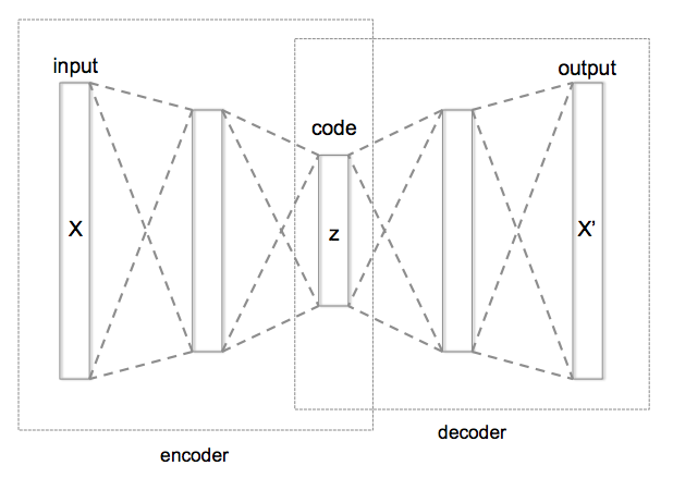
Autoencoder是一種可以將資料中的重要資訊保留下來的神經網路，有點像是資料壓縮，在做資料壓縮時，會有一個 Encoder 可以壓縮資料，另外還有一個 Decoder，可以還原資料。壓縮的過程就是用更精簡的方式保存了資料。Autoencoder 跟一般資料壓縮類似，也有 Encoder和Decoder，但 Decoder 的結果，不能確保可以完全還原。

Autoencoder會試著從測試資料，自己學習出Encoder和Decoder，並盡量讓資料在壓縮後又可以還原回去。實際上最常見的應用是，對圖片進行降噪 DeNoise。Autoencoder 是一種資料壓縮/解壓縮演算法，能夠處理 (1) 特定資料 (2) 壓縮後會遺失部分資訊，也就是無法完整還原回原本的資料 (3) 可由訓練資料中自動學習壓縮的方法。特定資料的意思跟常見的語音壓縮 mp3 不同，MPEG-2 Audio Layer III (mp3)，可以處理所有的語音資料，但 AutoEncoder 訓練的結果，只能處理跟訓練資料類似的語音資料。例如處理人臉圖片的 autoencoder，無法有效處理 tree 的圖片。

不管是「Encoder」還是「Decoder」都可以調整權重，如果將Encoder+Decoder的結構建立好並搭配Input當作Output的目標答案，在訓練的過程中，Autoencoder會試著找出最好的權重來使得資訊可以盡量完整還原回去，換句話說，Autoencoder可以自行找出了Encoder和Decoder。

Encoder 的效果等同於做 Dimension Reduction，Encoder會轉換原本的資料到一個新的空間，這個空間可以比原本Features描述的空間更能精簡的描述這群數據，而中間這層Layer的數值Embedding Code就是新空間裡頭的座標，有些時候我們會用這個新空間來判斷每筆資料之間的接近程度。

理論上是無法做出一個 autoencoder，其得到的壓縮效果，能夠跟類似 jpeg, mp3 這種壓縮方法一樣好，因為我們無法取得「所有」的語音/圖片資料，進行訓練。

目前 autoencoder 有兩個實用的應用：(1) data denoising 例如圖片降噪 (2) dimensionality reduction for data visulization 對於多維度離散的資料，autoencoder 能夠學習出 data projection，功能跟 PCA (Principla Compoenent Analysis) 或 t-SNE 一樣，但效果更好。（ref: 淺談降維方法中的 PCA 與 t-SNE）

Simple Autoencoder

# -*- coding: utf-8 -*-
from keras.datasets import mnist
from keras.utils import np_utils
import numpy as np
np.random.seed(10)

# 讀取 mnist 資料
(x_train, y_train), (x_test, y_test) = mnist.load_data()

# 標準化
x_train = x_train.astype('float32') / 255.
x_test = x_test.astype('float32') / 255.

# 正規化資料維度，以便 Keras 處理
x_train = x_train.reshape((len(x_train), np.prod(x_train.shape[1:])))
x_test = x_test.reshape((len(x_test), np.prod(x_test.shape[1:])))

print("x_train.shape=",x_train.shape, ", x_test.shape=",x_test.shape)

# simple autoencoder
# 建立 Autoencoder Model 並使用 x_train 資料進行訓練
from keras.layers import Input, Dense
from keras.models import Model

# this is the size of our encoded representations
encoding_dim = 32  # 32 floats -> compression of factor 24.5, assuming the input is 784 floats

# this is our input placeholder
input_img = Input(shape=(784,))
# "encoded" is the encoded representation of the input
encoded = Dense(encoding_dim, activation='relu')(input_img)
# "decoded" is the lossy reconstruction of the input
decoded = Dense(784, activation='sigmoid')(encoded)

# 建立 Model 並將 loss funciton 設為 binary cross entropy
# this model maps an input to its reconstruction
autoencoder = Model(input_img, decoded)
autoencoder.compile(optimizer='adadelta', loss='binary_crossentropy')

autoencoder.fit(x_train,
                x_train,  # Label 也設為 x_train
                epochs=25,
                batch_size=128,
                shuffle=True,
                validation_data=(x_test, x_test))

##########
# 另外製作 encoder, decoder 兩個分開的 Model
# this model maps an input to its encoded representation
encoder = Model(input_img, encoded)

# create a placeholder for an encoded (32-dimensional) input
encoded_input = Input(shape=(encoding_dim,))
# retrieve the last layer of the autoencoder model
decoder_layer = autoencoder.layers[-1]
# create the decoder model
decoder = Model(encoded_input, decoder_layer(encoded_input))

# encode and decode some digits
# note that we take them from the *test* set
encoded_imgs = encoder.predict(x_test)
decoded_imgs = decoder.predict(encoded_imgs)

# use Matplotlib
import matplotlib
matplotlib.use('agg')

import matplotlib.pyplot as plt
plt.clf()
n = 10  # how many digits we will display
plt.figure(figsize=(20, 4))
for i in range(n):
    # display original
    ax = plt.subplot(2, n, i + 1)
    plt.imshow(x_test[i].reshape(28, 28))
    plt.gray()
    ax.get_xaxis().set_visible(False)
    ax.get_yaxis().set_visible(False)

    # display reconstruction
    ax = plt.subplot(2, n, i + 1 + n)
    plt.imshow(decoded_imgs[i].reshape(28, 28))
    plt.gray()
    ax.get_xaxis().set_visible(False)
    ax.get_yaxis().set_visible(False)
plt.savefig("auto.png")

訓練過程

60000/60000 [==============================] - 4s 62us/step - loss: 0.3079 - val_loss: 0.2502
Epoch 2/25
60000/60000 [==============================] - 1s 12us/step - loss: 0.2300 - val_loss: 0.2105
Epoch 3/25
60000/60000 [==============================] - 1s 12us/step - loss: 0.2009 - val_loss: 0.1898
Epoch 4/25
60000/60000 [==============================] - 1s 13us/step - loss: 0.1839 - val_loss: 0.1756
Epoch 5/25
60000/60000 [==============================] - 1s 14us/step - loss: 0.1715 - val_loss: 0.1650
Epoch 6/25
60000/60000 [==============================] - 1s 13us/step - loss: 0.1619 - val_loss: 0.1563
Epoch 7/25
60000/60000 [==============================] - 1s 12us/step - loss: 0.1540 - val_loss: 0.1490
Epoch 8/25
60000/60000 [==============================] - 1s 12us/step - loss: 0.1473 - val_loss: 0.1429
Epoch 9/25
60000/60000 [==============================] - 1s 12us/step - loss: 0.1415 - val_loss: 0.1373
Epoch 10/25
60000/60000 [==============================] - 1s 12us/step - loss: 0.1365 - val_loss: 0.1325
Epoch 11/25
60000/60000 [==============================] - 1s 12us/step - loss: 0.1320 - val_loss: 0.1282
Epoch 12/25
60000/60000 [==============================] - 1s 12us/step - loss: 0.1279 - val_loss: 0.1243
Epoch 13/25
60000/60000 [==============================] - 1s 12us/step - loss: 0.1242 - val_loss: 0.1208
Epoch 14/25
60000/60000 [==============================] - 1s 12us/step - loss: 0.1209 - val_loss: 0.1178
Epoch 15/25
60000/60000 [==============================] - 1s 12us/step - loss: 0.1180 - val_loss: 0.1151
Epoch 16/25
60000/60000 [==============================] - 1s 12us/step - loss: 0.1155 - val_loss: 0.1127
Epoch 17/25
60000/60000 [==============================] - 1s 12us/step - loss: 0.1133 - val_loss: 0.1107
Epoch 18/25
60000/60000 [==============================] - 1s 12us/step - loss: 0.1115 - val_loss: 0.1090
Epoch 19/25
60000/60000 [==============================] - 1s 12us/step - loss: 0.1098 - val_loss: 0.1075
Epoch 20/25
60000/60000 [==============================] - 1s 12us/step - loss: 0.1085 - val_loss: 0.1062
Epoch 21/25
60000/60000 [==============================] - 1s 12us/step - loss: 0.1073 - val_loss: 0.1051
Epoch 22/25
60000/60000 [==============================] - 1s 14us/step - loss: 0.1062 - val_loss: 0.1042
Epoch 23/25
60000/60000 [==============================] - 1s 13us/step - loss: 0.1053 - val_loss: 0.1033
Epoch 24/25
60000/60000 [==============================] - 1s 15us/step - loss: 0.1046 - val_loss: 0.1026
Epoch 25/25
60000/60000 [==============================] - 1s 12us/step - loss: 0.1039 - val_loss: 0.1020

這是測試的前10 筆資料，上面是原始測試圖片，下面是經過壓縮/解壓縮後，產生的圖片，因為是簡單的 autoencoder，目前的效果還不夠好。

Sparse Autoencoder

ref: Tensorflow Day17 Sparse Autoencoder

在 encoded representation 加上 sparsity constraint

原本只有限制 hidden layer 為 32 維，在 hidden representation 加上 sparsity constraint。原本所有神經元會對所有輸入資料都有反應，但我們希望神經元只對某一些訓練資料有反應，例如神經元 A 對 5 有反應，B 只對 7 有反應。讓神經元有對每一個數字都有專業工作。

可在 loss function 加上兩項，達到這個限制

Sparsity Regularization
L2 Regularization

將 activity_regularizer 增加到 Dense Layer，並將訓練次數改為 100 次（因為增加了constraint，可以訓練更多次，而不會發生 overfitting）

# this is our input placeholder
input_img = Input(shape=(784,))
# "encoded" is the encoded representation of the input
# add a Dense layer with a L1 activity regularizer
encoded = Dense(encoding_dim, activation='relu',
                activity_regularizer=regularizers.l1(10e-5))(input_img)

# "decoded" is the lossy reconstruction of the input
decoded = Dense(784, activation='sigmoid')(encoded)

Note: 實際上這個部分測試的結果，反而變更差，目前不知道原因

Epoch 100/100
60000/60000 [==============================] - 1s 12us/step - loss: 0.2612 - val_loss: 0.2603

Deep AutoEncoder

在 encoded, decoded 從原本的一層，改為 3 層

# -*- coding: utf-8 -*-
from keras.datasets import mnist
from keras.utils import np_utils
import numpy as np
np.random.seed(10)

# 讀取 mnist 資料
(x_train, y_train), (x_test, y_test) = mnist.load_data()

# 標準化
x_train = x_train.astype('float32') / 255.
x_test = x_test.astype('float32') / 255.

# 正規化資料維度，以便 Keras 處理
x_train = x_train.reshape((len(x_train), np.prod(x_train.shape[1:])))
x_test = x_test.reshape((len(x_test), np.prod(x_test.shape[1:])))

print("x_train.shape=",x_train.shape, ", x_test.shape=",x_test.shape)

# simple autoencoder
# 建立 Autoencoder Model 並使用 x_train 資料進行訓練
from keras.layers import Input, Dense
from keras.models import Model
from keras import regularizers

# this is the size of our encoded representations
encoding_dim = 32  # 32 floats -> compression of factor 24.5, assuming the input is 784 floats

input_img = Input(shape=(784,))
encoded = Dense(128, activation='relu')(input_img)
encoded = Dense(64, activation='relu')(encoded)
encoded = Dense(32, activation='relu')(encoded)

decoded = Dense(64, activation='relu')(encoded)
decoded = Dense(128, activation='relu')(decoded)
decoded = Dense(784, activation='sigmoid')(decoded)

# 建立 Model 並將 loss funciton 設為 binary cross entropy
# this model maps an input to its reconstruction
autoencoder = Model(input_img, decoded)
autoencoder.compile(optimizer='adadelta', loss='binary_crossentropy')

autoencoder.fit(x_train,
                x_train,  # Label 也設為 x_train
                epochs=100,
                batch_size=128,
                shuffle=True,
                validation_data=(x_test, x_test))


# _________________________________________________________________
# Layer (type)                 Output Shape              Param #
# =================================================================
# input_1 (InputLayer)         (None, 784)               0
# _________________________________________________________________
# dense_1 (Dense)              (None, 128)               100480
# _________________________________________________________________
# dense_2 (Dense)              (None, 64)                8256
# _________________________________________________________________
# dense_3 (Dense)              (None, 32)                2080
# _________________________________________________________________
# dense_4 (Dense)              (None, 64)                2112
# _________________________________________________________________
# dense_5 (Dense)              (None, 128)               8320
# _________________________________________________________________
# dense_6 (Dense)              (None, 784)               101136
# =================================================================
# Total params: 222,384
# Trainable params: 222,384
# Non-trainable params: 0

decoded_imgs = autoencoder.predict(x_test)

# use Matplotlib
import matplotlib
matplotlib.use('agg')

import matplotlib.pyplot as plt
plt.clf()
n = 10  # how many digits we will display
plt.figure(figsize=(20, 4))
for i in range(n):
    # display original
    ax = plt.subplot(2, n, i + 1)
    plt.imshow(x_test[i].reshape(28, 28))
    plt.gray()
    ax.get_xaxis().set_visible(False)
    ax.get_yaxis().set_visible(False)

    # display reconstruction
    ax = plt.subplot(2, n, i + 1 + n)
    plt.imshow(decoded_imgs[i].reshape(28, 28))
    plt.gray()
    ax.get_xaxis().set_visible(False)
    ax.get_yaxis().set_visible(False)
plt.savefig("auto.png")

訓練結果 loss rate 由 0.1 降到 0.09

Epoch 100/100
60000/60000 [==============================] - 2s 33us/step - loss: 0.0927 - val_loss: 0.0925

Convolutional Autoencoder

執行前要加上環境變數

export TF_FORCE_GPU_ALLOW_GROWTH=true

執行結果

Epoch 50/50
60000/60000 [==============================] - 3s 57us/step - loss: 0.1012 - val_loss: 0.0984

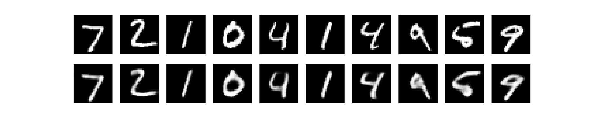
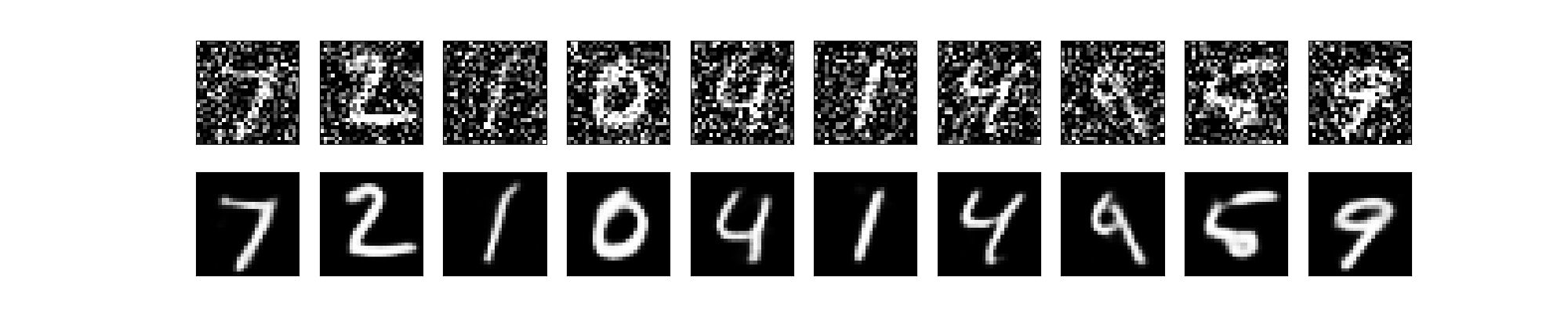
Image Denoise

用加上 noise 的圖片當作 input，output 為沒有 noise 的圖片，這樣進行 model 訓練

# -*- coding: utf-8 -*-
from keras.datasets import mnist
from keras.utils import np_utils
import numpy as np
np.random.seed(10)

# 讀取 mnist 資料
(x_train, y_train), (x_test, y_test) = mnist.load_data()

# 標準化
x_train = x_train.astype('float32') / 255.
x_test = x_test.astype('float32') / 255.

# 正規化資料維度，以便 Keras 處理
x_train = np.reshape(x_train, (len(x_train), 28, 28, 1))  # adapt this if using `channels_first` image data format
x_test = np.reshape(x_test, (len(x_test), 28, 28, 1))  # adapt this if using `channels_first` image data format


# 將原圖加上 noise
noise_factor = 0.5
x_train_noisy = x_train + noise_factor * np.random.normal(loc=0.0, scale=1.0, size=x_train.shape)
x_test_noisy = x_test + noise_factor * np.random.normal(loc=0.0, scale=1.0, size=x_test.shape)

x_train_noisy = np.clip(x_train_noisy, 0., 1.)
x_test_noisy = np.clip(x_test_noisy, 0., 1.)


print("x_train.shape=",x_train.shape, ", x_test.shape=",x_test.shape)

from keras.layers import Input, Dense, Conv2D, MaxPooling2D, UpSampling2D
from keras.models import Model
from keras import backend as K

input_img = Input(shape=(28, 28, 1))  # adapt this if using `channels_first` image data format

## model

x = Conv2D(32, (3, 3), activation='relu', padding='same')(input_img)
x = MaxPooling2D((2, 2), padding='same')(x)
x = Conv2D(32, (3, 3), activation='relu', padding='same')(x)
encoded = MaxPooling2D((2, 2), padding='same')(x)

# at this point the representation is (7, 7, 32)

x = Conv2D(32, (3, 3), activation='relu', padding='same')(encoded)
x = UpSampling2D((2, 2))(x)
x = Conv2D(32, (3, 3), activation='relu', padding='same')(x)
x = UpSampling2D((2, 2))(x)
decoded = Conv2D(1, (3, 3), activation='sigmoid', padding='same')(x)

autoencoder = Model(input_img, decoded)

autoencoder.compile(optimizer='adadelta', loss='binary_crossentropy')

autoencoder.fit(x_train_noisy,
                x_train,  # Label 也設為 x_train
                epochs=100,
                batch_size=128,
                shuffle=True,
                validation_data=(x_test_noisy, x_test))


decoded_imgs = autoencoder.predict(x_test_noisy)

# use Matplotlib
import matplotlib
matplotlib.use('agg')

import matplotlib.pyplot as plt
plt.clf()
n = 10  # how many digits we will display
plt.figure(figsize=(20, 4))
for i in range(n):
    # display original
    ax = plt.subplot(2, n, i + 1)
    plt.imshow(x_test_noisy[i].reshape(28, 28))
    plt.gray()
    ax.get_xaxis().set_visible(False)
    ax.get_yaxis().set_visible(False)

    # display reconstruction
    ax = plt.subplot(2, n, i + 1 + n)
    plt.imshow(decoded_imgs[i].reshape(28, 28))
    plt.gray()
    ax.get_xaxis().set_visible(False)
    ax.get_yaxis().set_visible(False)
plt.savefig("auto.png")

結果

Epoch 100/100
60000/60000 [==============================] - 3s 56us/step - loss: 0.0941 - val_loss: 0.0941

Sequence-to-sequence Autoencoder

如果輸入的資料是 sequence，而不是 vector / 2D image，如果想要有 temporal structure 的 model 要改用 LSTM

from keras.layers import Input, LSTM, RepeatVector
from keras.models import Model

inputs = Input(shape=(timesteps, input_dim))
encoded = LSTM(latent_dim)(inputs)

decoded = RepeatVector(timesteps)(encoded)
decoded = LSTM(input_dim, return_sequences=True)(decoded)

sequence_autoencoder = Model(inputs, decoded)
encoder = Model(inputs, encoded)