
tensorflow 的 MNIST 資料及共有訓練資料 55000 筆,驗證資料 5000筆,每一筆資料由 feature (影像)與 label (數字) 組成。
注意:要改用 tensorflow.keras.datasets
tensorflow.examples.tutorials is now deprecated and it is recommended to use tensorflow.keras.datasetsMNIST 資料處理
import tensorflow as tf
import numpy as np

mnist = tf.keras.datasets.mnist
# Tuple of Numpy arrays: (x_train, y_train), (x_test, y_test)

(x_train, y_train), (x_test, y_test) = mnist.load_data()
# 將每個 pixel 的值從 Int 轉成 floating point 同時做normalize(這是很常見的preprocessing)
# x_train, x_test = x_train / 255.0, x_test / 255.0

# 查看 train Data
print('x_train length = ', len(x_train), ', x_test length = ', len(x_test))
# x_train length =  60000 , x_test length =  10000
print('x_train.shape = ', x_train.shape, ', x_train[0].shape = ', x_train[0].shape, ', x_test[0].shape=', x_test[0].shape)
# 每張圖片 大小為 28x28
# x_train.shape =  (60000, 28, 28) , x_train[0].shape =  (28, 28) , x_test[0].shape= (28, 28)

print('x_train[0].length = ', len(x_train[0]) )
# x_train[0].length =  28
print('y_train length = ', len(y_train), ', y_train[0] = ', y_train[0])
# y_train length =  60000 , y_train[0] =  5


# 將 第一張 x_train 的圖片儲存到檔案
import matplotlib.pyplot as plt
def plot_image(image, filename):
    plt.clf()
    plt.imshow(image.reshape(28,28), cmap='binary')
    plt.savefig(filename)
plot_image(x_train[0], "x_train_index_0.png")


# 將 training 的 input 資料 28*28 的 2維陣列 轉為 1維陣列,再轉成 float32
# 每一個圖片,都變成 784 個 float 的 array
# training 與 testing 資料數量分別是 60000 與 10000 筆
# X_train_2D 是 [60000, 28*28] 的 2維陣列
x_train_2D = x_train.reshape(60000, 28*28).astype('float32')
x_test_2D = x_test.reshape(10000, 28*28).astype('float32')
print('x_train_2D.shape=', x_train_2D.shape)
# x_train_2D.shape=(60000, 784)


# 將圖片的數字 (0~255) 標準化,最簡單的方法就是直接除以 255
# x_train_norm 是標準化後的結果,每一個數字介於 0~1 之間
x_train_norm = x_train_2D/255
x_test_norm = x_test_2D/255

# 將 training 的 label 進行 one-hot encoding,例如數字 7 經過 One-hot encoding 轉換後是 array([0., 0., 0., 0., 0., 0., 0., 1., 0., 0.], dtype=float32),即第7個值為 1

one_hot=tf.one_hot(y_train,10)

with tf.compat.v1.Session() as sess:
    init = tf.compat.v1.global_variables_initializer()
    sess.run(init)
    y_train_one_hot = sess.run(one_hot)

    print( y_train_one_hot )
    print( 'y_train[0] = ', y_train[0], ", y_train_one_hot[0]=", y_train_one_hot[0] )
    # y_train[0] =  5 , y_train_one_hot[0]= [0. 0. 0. 0. 0. 1. 0. 0. 0. 0.]

    # 也可以用 np.argmax 將 one_hot 陣列,轉換回原本的數字
    print( 'y_train[0] = ', np.argmax(y_train_one_hot[0]) )
    # y_train[0] =  5

    # 列印前10筆 one hot
    for i in range(10):
        print(y_train_one_hot[i])
        # [0. 0. 0. 0. 0. 1. 0. 0. 0. 0.]
        # [1. 0. 0. 0. 0. 0. 0. 0. 0. 0.]
        # [0. 0. 0. 0. 1. 0. 0. 0. 0. 0.]
        # [0. 1. 0. 0. 0. 0. 0. 0. 0. 0.]
        # [0. 0. 0. 0. 0. 0. 0. 0. 0. 1.]
        # [0. 0. 1. 0. 0. 0. 0. 0. 0. 0.]
        # [0. 1. 0. 0. 0. 0. 0. 0. 0. 0.]
        # [0. 0. 0. 1. 0. 0. 0. 0. 0. 0.]
        # [0. 1. 0. 0. 0. 0. 0. 0. 0. 0.]
        # [0. 0. 0. 0. 1. 0. 0. 0. 0. 0.]
用一個 function 列印多筆圖片, label 資訊
import tensorflow as tf
import numpy as np

mnist = tf.keras.datasets.mnist
# Tuple of Numpy arrays: (x_train, y_train), (x_test, y_test)

(x_train, y_train), (x_test, y_test) = mnist.load_data()

# 將 training 的 input 資料 28*28 的 2維陣列 轉為 1維陣列,再轉成 float32
# 每一個圖片,都變成 784 個 float 的 array
# training 與 testing 資料數量分別是 60000 與 10000 筆
# X_train_2D 是 [60000, 28*28] 的 2維陣列
x_train_2D = x_train.reshape(60000, 28*28).astype('float32')
x_test_2D = x_test.reshape(10000, 28*28).astype('float32')
print('x_train_2D.shape=', x_train_2D.shape)
# x_train_2D.shape=(60000, 784)

# 將圖片的數字 (0~255) 標準化,最簡單的方法就是直接除以 255
# x_train_norm 是標準化後的結果,每一個數字介於 0~1 之間
x_train_norm = x_train_2D/255
x_test_norm = x_test_2D/255

# 將 training 的 label 進行 one-hot encoding,例如數字 7 經過 One-hot encoding 轉換後是 array([0., 0., 0., 0., 0., 0., 0., 1., 0., 0.], dtype=float32),即第7個值為 1

y_train_one_hot_tf=tf.one_hot(y_train,10)
y_test_one_hot_tf=tf.one_hot(y_test,10)

with tf.compat.v1.Session() as sess:
    init = tf.compat.v1.global_variables_initializer()
    sess.run(init)
    y_train_one_hot = sess.run(y_train_one_hot_tf)
    y_test_one_hot = sess.run(y_test_one_hot_tf)


# 查看多筆資料,以及 label
import matplotlib.pyplot as plt
def plot_images_labels_prediction(images,labels,prediction,idx,filename, num=10):
    fig = plt.gcf()
    fig.set_size_inches(12, 14)
    if num>25: num=25
    for i in range(0, num):
        ax=plt.subplot(5,5, 1+i)

        # 將 images 的 784 個數字轉換為 28x28
        ax.imshow(np.reshape(images[idx],(28, 28)), cmap='binary')

        # 轉換 one_hot label 為數字
        title= "label=" +str(np.argmax(labels[idx]))
        if len(prediction)>0:
            title+=",predict="+str(prediction[idx])

        ax.set_title(title,fontsize=10)
        ax.set_xticks([]);ax.set_yticks([])
        idx+=1
    plt.savefig(filename)

plot_images_labels_prediction(x_train_2D, y_train_one_hot,[], 0, 'x_train_0.png', 10)
plot_images_labels_prediction(x_train_2D, y_train_one_hot,[], 10, 'x_train_1.png', 10)

plot_images_labels_prediction(x_test_2D, y_test_one_hot,[], 0, 'x_test_0.png', 10)
plot_images_labels_prediction(x_test_2D, y_test_one_hot,[], 10, 'x_test_1.png', 10)
以 tensorflow 建立 MLP
訓練部分資料共有 60000 筆,經過預處理後,會產生 feature, label,然後輸入 MLP model 進行訓練,訓練完成的模型,可在預測階段使用。
import tensorflow as tf
import numpy as np
# STEP 1 讀取資料
mnist = tf.keras.datasets.mnist
# Tuple of Numpy arrays: (x_train, y_train), (x_test, y_test)
(x_train, y_train), (x_test, y_test) = mnist.load_data()
# 將 training 的 input 資料 28*28 的 2維陣列 轉為 1維陣列,再轉成 float32
# 每一個圖片,都變成 784 個 float 的 array
# training 與 testing 資料數量分別是 60000 與 10000 筆
# X_train_2D 是 [60000, 28*28] 的 2維陣列
x_train_2D = x_train.reshape(60000, 28*28).astype('float32')
x_test_2D = x_test.reshape(10000, 28*28).astype('float32')
print('x_train_2D.shape=', x_train_2D.shape)
# x_train_2D.shape=(60000, 784)
# 將圖片的數字 (0~255) 標準化,最簡單的方法就是直接除以 255
# x_train_norm 是標準化後的結果,每一個數字介於 0~1 之間
x_train_norm = x_train_2D/255
x_test_norm = x_test_2D/255
# 將 training 的 label 進行 one-hot encoding,例如數字 7 經過 One-hot encoding 轉換後是 array([0., 0., 0., 0., 0., 0., 0., 1., 0., 0.], dtype=float32),即第7個值為 1
y_train_one_hot_tf=tf.one_hot(y_train,10)
y_test_one_hot_tf=tf.one_hot(y_test,10)
y_train_one_hot = None
y_test_one_hot = None
with tf.compat.v1.Session() as sess:
init = tf.compat.v1.global_variables_initializer()
sess.run(init)
y_train_one_hot = sess.run(y_train_one_hot_tf)
y_test_one_hot = sess.run(y_test_one_hot_tf)
# 將 x_train, y_train 分成 train 與 validation 兩個部分
x_train_norm_data = x_train_norm[0:50000]
x_train_norm_validation = x_train_norm[50000:60000]
y_train_one_hot_data = y_train_one_hot[0:50000]
y_train_one_hot_validation = y_train_one_hot[50000:60000]
### 建立模型
# keras 只需要用 model = Sequential() 建立線性堆疊模型,再用 model.add() 將各神經網路層加入模型,但 tensorflow 需要自己定義 layer 函數
def layer(output_dim,input_dim,inputs, activation=None):
W = tf.Variable(tf.random.normal([input_dim, output_dim]))
b = tf.Variable(tf.random.normal([1, output_dim]))
XWb = tf.matmul(inputs, W) + b
if activation is None:
outputs = XWb
else:
outputs = activation(XWb)
return outputs
# 輸入層, 784 個神經元, 資料型別為 float
# 第一維是 None,因為輸入資料的筆數還不確定,所以設定為 None
# 第二維是 784,因為每個圖片是 784 個像素點
x = tf.compat.v1.placeholder("float", [None, 784])
# 隱藏層, 256 個神經元
h1=layer(output_dim=256,input_dim=784, inputs=x ,activation=tf.nn.relu)
# 輸出層, 10 個神經元
y_predict=layer(output_dim=10,input_dim=256, inputs=h1,activation=None)
#### 定義訓練方式
# keras 要用 model.compile,設定 loss function 及 optimizer 與 metrics 設定評估模型的方法
# tensorflow 需要自己定義 loass function、最優化方法 optimizer,及設定參數,以及定義評估模型準確率的公式
# 建立訓練資料 label 真實值 placeholder
y_label = tf.compat.v1.placeholder("float", [None, 10])
# 定義loss function
loss_function = tf.reduce_mean(
tf.nn.softmax_cross_entropy_with_logits
(logits=y_predict ,
labels=y_label))
# 選擇optimizer
optimizer = tf.compat.v1.train.AdamOptimizer(learning_rate=0.001).minimize(loss_function)
### 定義評估模型的準確率
#計算每一筆資料是否正確預測
correct_prediction = tf.equal(tf.argmax(y_label , 1),
tf.argmax(y_predict, 1))
#將計算預測正確結果,加總平均
accuracy = tf.reduce_mean(tf.cast(correct_prediction, "float"))
### 訓練模型
trainEpochs = 15
batchSize = 100
totalBatchs = int(len(x_train_norm_data)/batchSize)
epoch_list=[];loss_list=[];accuracy_list=[]
from time import time
with tf.compat.v1.Session() as sess:
startTime=time()
sess.run(tf.compat.v1.global_variables_initializer())
for epoch in range(trainEpochs):
for i in range(totalBatchs):
# batch_x, batch_y = mnist.train.next_batch(batchSize)
batch_x = x_train_norm_data[i*batchSize:(i+1)*batchSize]
batch_y = y_train_one_hot_data[i*batchSize:(i+1)*batchSize]
sess.run(optimizer,feed_dict={x: batch_x,y_label: batch_y})
# loss,acc = sess.run([loss_function,accuracy],
# feed_dict={x: mnist.validation.images,
# y_label: mnist.validation.labels})
loss,acc = sess.run([loss_function,accuracy],
feed_dict={x: x_train_norm_validation,
y_label: y_train_one_hot_validation})
epoch_list.append(epoch);loss_list.append(loss)
accuracy_list.append(acc)
print("Train Epoch:", '%02d' % (epoch+1), "Loss=", "{:.9f}".format(loss)," Accuracy=",acc)
duration =time()-startTime
print("Train Finished takes:",duration)
### 評估模型準確率
print("Accuracy:", sess.run(accuracy,
feed_dict={x: x_test_norm,
y_label: y_test_one_hot}))
### 進行預測
prediction_result=sess.run(tf.argmax(y_predict,1),
feed_dict={x: x_test_norm })
# matplotlib 列印 loss, accuracy 折線圖
import matplotlib.pyplot as plt
fig = plt.gcf()
# fig.set_size_inches(4,2)
plt.plot(epoch_list, loss_list, label = 'loss')
plt.ylabel('loss')
plt.xlabel('epoch')
plt.legend(['loss'], loc='upper left')
plt.savefig('loss.png')
fig = plt.gcf()
# fig.set_size_inches(4,2)
plt.plot(epoch_list, accuracy_list,label="accuracy" )
plt.ylim(0.8,1)
plt.ylabel('accuracy')
plt.xlabel('epoch')
plt.legend(['accuracy'], loc='upper right')
plt.savefig('accuracy.png')
############
# 查看多筆資料,以及 label
import matplotlib.pyplot as plt
def plot_images_labels_prediction(images,labels,prediction,idx,filename, num=10):
fig = plt.gcf()
fig.set_size_inches(12, 14)
if num>25: num=25
for i in range(0, num):
ax=plt.subplot(5,5, 1+i)
# 將 images 的 784 個數字轉換為 28x28
ax.imshow(np.reshape(images[idx],(28, 28)), cmap='binary')
# 轉換 one_hot label 為數字
title= "label=" +str(np.argmax(labels[idx]))
if len(prediction)>0:
title+=",predict="+str(prediction[idx])
ax.set_title(title,fontsize=10)
ax.set_xticks([]);ax.set_yticks([])
idx+=1
plt.savefig(filename)
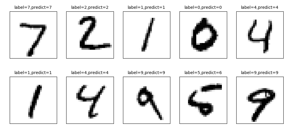
plot_images_labels_prediction(x_test_norm,
y_test_one_hot,
prediction_result,0, "result.png", num=10)
# 找出預測錯誤
for i in range(400):
if prediction_result[i]!=np.argmax(y_test_one_hot[i]):
print("i="+str(i)+
" label=",np.argmax(y_test_one_hot[i]),
"predict=",prediction_result[i])
Train Epoch: 01 Loss= 6.828331470  Accuracy= 0.8309
Train Epoch: 02 Loss= 4.488496780  Accuracy= 0.8758
Train Epoch: 03 Loss= 3.577744246  Accuracy= 0.8964
Train Epoch: 04 Loss= 3.057111502  Accuracy= 0.9064
Train Epoch: 05 Loss= 2.736637831  Accuracy= 0.9137
Train Epoch: 06 Loss= 2.479548931  Accuracy= 0.9204
Train Epoch: 07 Loss= 2.278975010  Accuracy= 0.9226
Train Epoch: 08 Loss= 2.162630558  Accuracy= 0.9254
Train Epoch: 09 Loss= 2.005532503  Accuracy= 0.9295
Train Epoch: 10 Loss= 1.911731601  Accuracy= 0.9324
Train Epoch: 11 Loss= 1.785833955  Accuracy= 0.9351
Train Epoch: 12 Loss= 1.694522023  Accuracy= 0.9371
Train Epoch: 13 Loss= 1.660093784  Accuracy= 0.9362
Train Epoch: 14 Loss= 1.623517632  Accuracy= 0.938
Train Epoch: 15 Loss= 1.616030455  Accuracy= 0.9384
Train Finished takes: 36.676905393600464
Accuracy: 0.9361

## 預測錯誤的圖片
i=8   label= 5 predict= 6
i=33   label= 4 predict= 0
i=41   label= 7 predict= 3
i=59   label= 5 predict= 8
i=63   label= 3 predict= 2
i=78   label= 9 predict= 7
i=115   label= 4 predict= 6
i=121   label= 4 predict= 8
i=126   label= 0 predict= 2
i=175   label= 7 predict= 2
i=215   label= 0 predict= 2
i=241   label= 9 predict= 8
i=247   label= 4 predict= 2
i=282   label= 7 predict= 8
i=290   label= 8 predict= 4
i=320   label= 9 predict= 8
i=321   label= 2 predict= 8
i=324   label= 0 predict= 8
i=325   label= 4 predict= 9
i=333   label= 5 predict= 3
i=359   label= 9 predict= 4
i=389   label= 9 predict= 4


將隱藏層的神經元由 256 改為 1000
# 隱藏層, 1000 個神經元
h1=layer(output_dim=1000,input_dim=784, inputs=x ,activation=tf.nn.relu)

# 輸出層, 10 個神經元
y_predict=layer(output_dim=10,input_dim=1000, inputs=h1,activation=None)
剛剛的正確率為
Accuracy: 0.9361改為 1000 後的正確率提升為
Accuracy: 0.95建立兩個隱藏層
x = tf.compat.v1.placeholder("float", [None, 784])

# 隱藏層 h1, 1000 個神經元
h1=layer(output_dim=1000,input_dim=784, inputs=x ,activation=tf.nn.relu)

# 隱藏層 h2, 1000 個神經元
h2=layer(output_dim=1000,input_dim=1000, inputs=h1 ,activation=tf.nn.relu)

# 輸出層, 10 個神經元
y_predict=layer(output_dim=10,input_dim=1000, inputs=h2,activation=None)
正確率可提升到
Accuracy: 0.9636
沒有留言:
張貼留言