2019/09/23

ZeroMQ

2010年3月30日,AMQP的最初設計者 iMatix 的執行長 Pieter Hintjens 宣布 iMatix 要退出AMQP工作群組,並實作簡單又快速的ZeroMQ,且不支援未來會發布的AMQP/1.0。針對 AMQP 的問題,在 iMatrix 的 What is wrong with AMQP 有說明他的論點。

ØMQ(也寫作ZeroMQ、0MQ或ZMQ) 是一個為可伸縮的分散式或並行應用程式設計的高效能非同步訊息庫,它提供一個訊息佇列的功能,但ZeroMQ 不需要專門的訊息代理(message broker) 就可以運作。 目前已經有很多不同的程式語言的函式庫可以使用,可參考 ØMQ Language Bindings 有不同程式語言 libray 的安裝方式。

安裝

在 mac 可用 macport 安裝,但這部分是要直接使用 C 語言開發的情況下才要安裝。

sudo port install zmq

如果要使用 python,可使用 ZeroMQ for python pyzmq 這個 library,他已經將 libzmq.so 包裝在裡面,因此直接安裝 pyzmq 就可以使用 ZeroMQ

sudo pip3 install pyzmq

安裝完成後,以一個簡單的範例測試

client.py

import zmq

context = zmq.Context()

socket = context.socket(zmq.REQ)
socket.connect ("tcp://127.0.0.1:7788")

socket.send(b'hello')
print( socket.recv() )

server.py

import zmq

context = zmq.Context()

socket = context.socket(zmq.REP)
socket.bind ("tcp://*:7788")

print( socket.recv() )
socket.send(b'world')

一般網路程式,都需要先啟動 server 後,才能啟動 client,不過 ØMQ 不同,不管誰先啟動都沒關係。以下是在兩個 terminal 分別執行 client/server 的結果。

$ python client.py
b'world'
$ python server.py
b'hello'

pyzmq 的所有 API 文件在 The PyZMQ API

加法計算的小程式

addserver.py

import os
import zmq

context = zmq.Context()

socket = context.socket(zmq.REP)
socket.connect("tcp://localhost:7788")

print( 'Worker %s is running ...' % os.getpid() )

while True:
    # receive request
    a, b = socket.recv_multipart()
    a = int(a)
    b = int(b)

    print( 'Compute %s + %s and send response' % (a, b) )
    socket.send_string( str(a + b) +" (from worker "+ str(os.getpid()) +")" )

addclient.py

import zmq
import random
import time

context = zmq.Context()

socket = context.socket(zmq.REQ)
socket.bind("tcp://*:7788")

# wait all worker connected
time.sleep(1)

for i in range(9):
    a = random.randint(0, 100)
    b = random.randint(0, 100)
    print( 'Compute %s + %s ...' % (a, b) )

    # send request to peer
    socket.send_multipart([bytes(str(a),"ascii"), bytes(str(b),"ascii")])

    # receive response from peer
    rep = socket.recv()
    print( ' = ' + rep.decode('UTF-8') )

在這裡例子必須先啟動 worker (addserver),我們先啟動三個 worker後,再啟動 addclient.py

$ python addserver.py
Worker 45777 is running ...
Compute 33 + 47 and send response
Compute 68 + 13 and send response
Compute 45 + 68 and send response

$ python addserver.py
Worker 45784 is running ...
Compute 69 + 88 and send response
Compute 86 + 13 and send response
Compute 22 + 8 and send response

$ python addserver.py
Worker 45792 is running ...
Compute 41 + 25 and send response
Compute 14 + 84 and send response
Compute 13 + 48 and send response

client 會用 send_multipart 的方式,將資料以 Round-Robin 方式平均分配給 workers,

$ python addclient.py
Compute 33 + 47 ...
 = 80 (from worker 45777)
Compute 41 + 25 ...
 = 66 (from worker 45792)
Compute 69 + 88 ...
 = 157 (from worker 45784)
Compute 68 + 13 ...
 = 81 (from worker 45777)
Compute 14 + 84 ...
 = 98 (from worker 45792)
Compute 86 + 13 ...
 = 99 (from worker 45784)
Compute 45 + 68 ...
 = 113 (from worker 45777)
Compute 13 + 48 ...
 = 61 (from worker 45792)
Compute 22 + 8 ...
 = 30 (from worker 45784)

如果刻意實作一個 addserver2.py,只服務一次計算,就中止 socket。

import os
import zmq

context = zmq.Context()

socket = None

try:
    socket = context.socket(zmq.REP)
    socket.connect("tcp://localhost:7788")

    print( 'Worker %s is running ...' % os.getpid() )

    # while True:
    # receive request
    a, b = socket.recv_multipart()
    a = int(a)
    b = int(b)

    print( 'Compute %s + %s and send response' % (a, b) )
    socket.send_string( str(a + b) +" (from worker "+ str(os.getpid()) +")" )
finally:
    if( socket is not None):
        socket.close()
    if( context is not None):
        context.term()

執行後可以發現,另外兩個 worker 有將其他的 task 處理掉,不過這時要注意,server2.py 在結束前一定要 close socket,否則 client 會一直在等待那一個 worker。

$ python addserver2.py
Worker 45982 is running ...
Compute 49 + 96 and send response

$ python addserver.py
Worker 45967 is running ...
Compute 47 + 63 and send response
Compute 49 + 74 and send response
Compute 69 + 78 and send response
Compute 29 + 10 and send response

$ python addserver.py
Worker 45974 is running ...
Compute 56 + 7 and send response
Compute 62 + 36 and send response
Compute 3 + 47 and send response
Compute 75 + 66 and send response


$ python addclient.py
Compute 47 + 63 ...
 = 110 (from worker 45967)
Compute 49 + 96 ...
 = 145 (from worker 45982)
Compute 56 + 7 ...
 = 63 (from worker 45974)
Compute 49 + 74 ...
 = 123 (from worker 45967)
Compute 62 + 36 ...
 = 98 (from worker 45974)
Compute 69 + 78 ...
 = 147 (from worker 45967)
Compute 3 + 47 ...
 = 50 (from worker 45974)
Compute 29 + 10 ...
 = 39 (from worker 45967)
Compute 75 + 66 ...
 = 141 (from worker 45974)

The Zen of Zero: Ø 的意義

ZeroMQ 的Zero 一開始代表 "zero broker",以及 "zero latency",後來慢慢增加了 "zero administration", "zero cost", "zero waste" 這些意思,也就是說,ZeroMQ 就是要盡可能降低複雜度。ZeroMQ 就像是增強功能的 socket library,也可以說是 mailboxes with routing。

我們再回到 ØMQ 的首頁,看一下這個專案的目標

  • Distributed Messaging: 也就是在分散式的環境,不僅是跨機器,也可以跨 process,跨 thread 進行通訊

  • 可以用多種程式語言在多種平台上互通訊息

  • 在 inproc, IPC, TCP, TIPC, multicast 這些情境中傳遞訊息

  • 支援 pub-sub, push-pull, and router-dealer 這些傳遞訊息的 pattern

  • 用極小的 library 提供高速非同步 I/O engines

  • 有很多開源社群的支援

  • 支援高階程式語言及平台

  • 可建立 centralized, distributed, small, or large 這些架構

  • 有商業支援的自由軟體

以下依照 ØMQ - The Guide in python 的說明瞭解 ØMQ,範例程式可以在 GitHub repository 取得。

ØMQ 收送資料的方法

Request-Reply

這是最基本的,Client 跟 Server 互相收送資料,client 會發送 "Hello" 給 server,server 回應 "World" 給 client。

hwserver.py 會 bind tcp port 5555,並在收到資料後,回應 "World"

import time
import zmq

context = zmq.Context()
socket = context.socket(zmq.REP)
socket.bind("tcp://*:5555")

while True:
    #  Wait for next request from client
    message = socket.recv()
    print("Received request: %s" % message)

    #  Do some 'work'
    time.sleep(1)

    #  Send reply back to client
    socket.send(b"World")

hwclient.py,會連接到 localhost:5555,會發送 10 次 "Hello",每一次發送後就會等待 server 回應。

import zmq

context = zmq.Context()

#  Socket to talk to server
print("Connecting to hello world server...")
socket = context.socket(zmq.REQ)
socket.connect("tcp://localhost:5555")

#  Do 10 requests, waiting each time for a response
for request in range(10):
    print("Sending request %s ..." % request)
    socket.send(b"Hello")

    #  Get the reply.
    message = socket.recv()
    print("Received reply %s [ %s ]" % (request, message))

我們可以先啟動 client,再啟動 server,或是同時啟動很多個 client。如果在 client 執行到一半,用 Ctrl-C 將 server 中斷,然後重新啟動 hwserver.py,會發現 client 並沒有繼續往下執行。這個問題會在 chap 4 Reliable Request-Reply Patterns 裡面討論。

Publish-Subscribe

剛剛的是 server-client 之間雙向的傳輸,第二種常見的 pattern 為單向的 data distribution,server 會持續發送資料給一些 clients。

wuserver.py 是天氣資訊 server 的範例,會持續一直發送資料,發送時會亂數處理一個 zipcode

#
#   Weather update server
#   Binds PUB socket to tcp://*:5556
#   Publishes random weather updates
#

import zmq
from random import randrange


context = zmq.Context()
socket = context.socket(zmq.PUB)
socket.bind("tcp://*:5556")

while True:
    zipcode = randrange(1, 100000)
    temperature = randrange(-80, 135)
    relhumidity = randrange(10, 60)

    socket.send_string("%i %i %i" % (zipcode, temperature, relhumidity))

wuclient.py 會透過 socket.setsockopt_string(zmq.SUBSCRIBE, zip_filter) 註冊只需要取得 zipcode 10001 的天氣資訊,程式後面取得五次天氣的更新資料,然後平均。

#
#   Weather update client
#   Connects SUB socket to tcp://localhost:5556
#   Collects weather updates and finds avg temp in zipcode
#

import sys
import zmq


#  Socket to talk to server
context = zmq.Context()
socket = context.socket(zmq.SUB)

print("Collecting updates from weather server...")
socket.connect("tcp://localhost:5556")

# Subscribe to zipcode, default is NYC, 10001
zip_filter = sys.argv[1] if len(sys.argv) > 1 else "10001"

# Python 2 - ascii bytes to unicode str
if isinstance(zip_filter, bytes):
    zip_filter = zip_filter.decode('ascii')
socket.setsockopt_string(zmq.SUBSCRIBE, zip_filter)

# Process 5 updates
total_temp = 0
for update_nbr in range(5):
    string = socket.recv_string()
    zipcode, temperature, relhumidity = string.split()
    total_temp += int(temperature)

print("Average temperature for zipcode '%s' was %dF" % (
      zip_filter, total_temp / (update_nbr+1))
)

SUB socket 必須要用 zmq_setsockopt() 設定要註冊取得的資訊是什麼,如果沒有註冊,就取不到任何資料。PUB-SUB socket pair 是非同步的。如果對 SUB socket 發送訊息(zmq_send()),就會發生 error,對 PUB socket 接收訊息(zmq_recv())也會發生 error。PUB socket 並不會理會有沒有 SUB socket 接收資料,會持續不斷發送資料出去。

另外,PUB-SUB sockets 中,不能保證 subscriber 什麼時候開始接收到訊息,就算是先啟動了 subscriber 再啟動 publisher,問題還是一樣會發生,subscriber 永遠會漏掉沒接收到 publisher 發送的第一個訊息。這是因為 subscriber 連接到 publisher 需要時間,但publisher 可能已經開始發送訊息了。

subscriber 並不能保證接收到所有 publisher 發送的訊息,在 chap2 會說明並解決這個問題。如果 publisher 有無限多的資料要發送給 subscriber,這個情境下,就不需要在意是不是接收到所有資料。

另外有一些要注意的事項:

  1. subscriber 可連接多個 publisher,資料會依次接收 (fair-queued),subscriber 不會一直接收到某一個 publisher 的資料
  2. 如果 publisher 沒有任何連接的 subscribers,就會直接丟棄所有訊息
  3. 如果是 TCP,且 subscriber 網路速度很慢,message 會被放在 publisher 的 queue,接下來會看到如何保護 publisher,解決這個問題

  4. 在 ØMQ 3.X 以後,如果是用 tcp:// 或是 ipc://,filter 會發生在 publisher 端,如果是用 epgm://,filter 會發生在 subscriber 端。在 2.X,所有 filtering 都發生在 subscriber 端。

Divide & Conquer - Parallel Pipeline

  • ventilator 會產生可平行處理得 tasks
  • 有多個 workers 處理 tasks
  • sink 會接收 worker 的處理結果

taskvent.py 會產生 100 個 tasks,在開始發送 task 之前,要先啟動某個數量的 worker

# Task ventilator
# Binds PUSH socket to tcp://localhost:5557
# Sends batch of tasks to workers via that socket

import zmq
import random
import time

try:
    raw_input
except NameError:
    # Python 3
    raw_input = input

context = zmq.Context()

# Socket to send messages on
sender = context.socket(zmq.PUSH)
sender.bind("tcp://*:5557")

# Socket with direct access to the sink: used to synchronize start of batch
sink = context.socket(zmq.PUSH)
sink.connect("tcp://localhost:5558")

print("Press Enter when the workers are ready: ")
_ = raw_input()
print("Sending tasks to workers...")

# The first message is "0" and signals start of batch
sink.send(b'0')

# Initialize random number generator
random.seed()

# Send 100 tasks
total_msec = 0
for task_nbr in range(100):

    # Random workload from 1 to 100 msecs
    workload = random.randint(1, 100)
    total_msec += workload

    sender.send_string(u'%i' % workload)

print("Total expected cost: %s msec" % total_msec)

# Give 0MQ time to deliver
time.sleep(1)

taskwork.py 取得 task 並 sleep 一段時間,然後發送完成的訊息

# Task worker
# Connects PULL socket to tcp://localhost:5557
# Collects workloads from ventilator via that socket
# Connects PUSH socket to tcp://localhost:5558
# Sends results to sink via that socket

import sys
import time
import zmq


context = zmq.Context()

# Socket to receive messages on
receiver = context.socket(zmq.PULL)
receiver.connect("tcp://localhost:5557")

# Socket to send messages to
sender = context.socket(zmq.PUSH)
sender.connect("tcp://localhost:5558")

# Process tasks forever
while True:
    s = receiver.recv()

    # Simple progress indicator for the viewer
    sys.stdout.write('.')
    sys.stdout.flush()

    # Do the work
    time.sleep(int(s)*0.001)

    # Send results to sink
    sender.send(b'')

tasksink.py,以 taskvent.py 發送的 b'0' 為啟動的訊號,接收 100 個 task 的結果,計算花費的時間

# Task sink
# Binds PULL socket to tcp://localhost:5558
# Collects results from workers via that socket
#
# Author: Lev Givon <lev(at)columbia(dot)edu>

import sys
import time
import zmq


context = zmq.Context()

# Socket to receive messages on
receiver = context.socket(zmq.PULL)
receiver.bind("tcp://*:5558")

# Wait for start of batch
s = receiver.recv()

# Start our clock now
tstart = time.time()

# Process 100 confirmations
for task_nbr in range(100):
    s = receiver.recv()
    if task_nbr % 10 == 0:
        sys.stdout.write(':')
    else:
        sys.stdout.write('.')
    sys.stdout.flush()

# Calculate and report duration of batch
tend = time.time()
print("Total elapsed time: %d msec" % ((tend-tstart)*1000))
  • worker 數量越多,處理完成的時間越短。
  • worker 上接 ventilator,下接 sink,數量可任意變動
  • ventilator 的 PUSH 會平均發送 task 給 workers,也稱為 load balancing
  • sink 的 PULL 會平均接收 workers 的結果,也稱為 fair queueing
  • 同樣會發生 "slow joiner" 的問題,會造成 load balancing 分配不均。如果某個 PULL socket 比較快 join,就會在其他 PULL socket 連接前,就先取得較多 task。如果需要較正確的 load balancing 機制,會在 chap3 Advanced Request-Reply Patterns 裡面說明。

ØMQ 的 string

ØMQ 在傳送資料時,必須要指定傳送的資料量,也就是說,我們要自己進行資料格式化。以 C 語言來說,string 是以 null byte 結束,因此可以這樣發送,也就是發送 6 bytes

zmq_send(requester, "Hello", 6, 0);

在 python 的 string 並沒有 null byte,因此在發送時,會在前面增加一個 byte 為字串長度

socket.send("Hello")

但如果在 C 語言接收 python 發送的資料,會發生沒有正確結束的字串的錯誤。因此最好的方式,是 allocate 新的 buffer,並增加一個 byte,複製 string 然後最後填上 null。以下 s_recv 只能處理 255 chars。

static char *
s_recv (void *socket) {
    char buffer [256];
    int size = zmq_recv (socket, buffer, 255, 0);
    if (size == -1)
        return NULL;
    if (size > 255)
        size = 255;
    buffer [size] = 0;
    return strdup (buffer);
}

ZeroMQ strings 是以指定長度的方式處理,發送時並不會在後面加上 null。

ØMQ 的版本

不同版本的 ØMQ 傳送資料可能會發生問題,以下是在 python 確認 ØMQ 版本資訊的方式,libzmq 的部分才是 ØMQ 的 library 的版本號碼。

import zmq

print("Current libzmq version is %s" % zmq.zmq_version())
print("Current  pyzmq version is %s" % zmq.__version__)

執行結果為

Current libzmq version is 4.2.5
Current  pyzmq version is 17.1.2

Programming in ØMQ

ØMQ 都是由取得 context 開始,然後 create socket,C語言是 zmq_ctx_new(),在 process 裡面只需要一個 context,因為 context 是單一 process 裡面所有 socket 的 container,並負責 inproc sockets 的傳輸工作,如果產生了兩個 context,就像是兩個獨立的 ØMQ instances。

在程式開始呼叫一次 zmq_ctx_new(),結束前呼叫一次 zmq_ctx_destroy()

如果有使用 fork() system call,每個 process 都需要自己的 context,如果在呼叫 fork 前先在 main process 呼叫 zmq_ctx_new(),每個 child process 都會取得自己的contexts,必須在 parent process 進行 context 管理。


python 有自動回收的功能,但 C 必須要自己回收 context,否則會產生 memory leak,如果讓 socket 維持 open,zmq_ctx_destory 會永遠停在那邊,等待 socket close。

使用 ØMQ 要注意的 objects 只有 messages, sockets, contexts

  • 盡可能使用 zmq_send(), zmq_recv(),可避免使用 zmq_msg_t objects

  • 如果使用 zmq_msg_recv(),必須要呼叫 zmq_msg_close() 用來 release the received message

  • 如果程式 opening/closing 很多 socket,可能需要 redesign application,這些 socket handles 會等到 context destory 才會被回收。

  • 離開 application 前,要先 close sockets,然後呼叫 zmq_ctx_destory()

如果是 python,會自動 destory object, socket, context,記得要放在 final block。

multithread 環境在下一章討論。

不要在多個 thread 裡面使用相同的 socket。

必須要設定 LINGER value (1 second) 然後 close socket

destroy context 會造成每個 thread 產生 blocking receives/polls/send,並會 return error,程式必須 catch error,設定 linger on, close socket 然後 exit。

不要呼叫兩次 destroy the same context,zmq_ctx_destory 會 block all sockets。

Why we needed ØMQ

application 需要處理訊息及 message queue,但常會自己利用 TCP/UDP 開發。

以下是一般 TCP 程式要注意的問題

  1. 如何處理 I/O?要在 application 或是背景處理 I/O?blocking I/O 的 architecture 並不 scalable,background I/O 很難設計

  2. 如何處理 dynamic components,如何區分 client/server 的 components

  3. 如何處理 message,如何設計容易 write/read 的資料格式,不會造成 buffer overflow

  4. 如何處理不能立即發送的訊息?尤其是在等待 component online 的時候,要丟棄訊息,放到資料庫或是放到 memory queue?

  5. 如何處理 message queue,當 reading 速度很慢,發生 queue 異常時要怎麼辦?

  6. 如何處理遺失的訊息?要等待 refresh,發送 resend或是建立 reliability layer,確保訊息一定會送達。

  7. 如果需要另一種 tranport layer 要怎麼辦?例如要用 multicast 取代 TCP,或是使用 IPv6

  8. 如何 route message,要重送相同的訊息給不同 peers,或是要發送 reply 給原本的 requester?

  9. 如何用不同程式語言撰寫 API?要重新實作 wire-level protocol,或要 repackage library?

  10. 如何在不同 architecture 讀取資料?如何設定 data type?

  11. 如何處理 network error

Hadoop Zookeeper 的 C API code 有 4200 lines 處理 client/server network communication protocol,且沒有文件,對其他開發者來說很難理解。

AMQP 試圖要用 "broker" 處理 addressing, routing, queueing,這會產生大量 client/server prototcol APIs。broker 對於大型網路來說,簡化了複雜度,但這會多了一個 black box,漸漸會讓 broker 變成另一個 bottleneck。需要另一個 team 去維護 broker,也需要 backup boxes。

ØMQ 的優勢

  1. 在 background thread 非同步處理 I/O,以 lock-free 方式跟 application thread 溝通。concurrent ØMQ 不需要 lock, semaphore, 或 wait states

  2. components 可隨時連線或斷線,ØMQ 會自動 reconnect,可用任意順序啟動 components

  3. 需要時會自動 queue message

  4. 有處理 over-full queue 的機制,當 queue full 時,ØMQ 會依照 pattern 決定要 block senders 或是丟棄 messages。

  5. 可使用 TCP, multicast, in-process, inter-process 的 transport layer

  6. 可處理 slow/blocked readers,依照不同 pattern 有不同處理方式

  7. 以 request-reply 或是 pub-sub 方式 route message

  8. 可用一個 function call,建立 proxies 用來 queue, forward, capture messages,proxies 可降低 network 互聯的複雜度

  9. 有保證訊息送達的機制

  10. 可以處理任意格式的訊息,可以是 msgpack, protocol buffers 或其他格式

  11. 可處理 network error

  12. 不需要太多運算資源

References

Learning ZeroMQ with pyzmq

新世紀通訊函式庫 – ZeroMQ

Learning and Using ØMQ http://zguide.zeromq.org

ØMQ - Get The Software

python zeromq安装

ØMQ - wiki

zeromq用來怎麼玩?

ZeroMQ 簡介

ZeroMQ Message Transport Protocol ZMTP 3.1

Easy cluster parallelization with ZeroMQ

2019/09/15

以 python 實作迴歸與分類程式

迴歸

學習資料

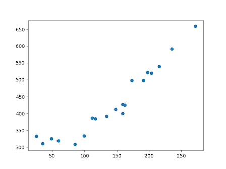
取得學習資料文字檔 click.csv

x,y
235,591
216,539
148,413
35,310
85,308
...

先利用 matplotlib 繪製到圖表上

import numpy as np
import matplotlib.pyplot as plt

train = np.loadtxt('click.csv', delimiter=',', skiprows=1)
train_x = train[:,0]
train_y = train[:,1]

plt.plot(train_x, train_y, 'o')
plt.show()

另外針對原始的學習資料,進行標準化(z-score正規化),也就是將資料平均轉換為 0,分散轉換為1。其中 𝜇 是所有資料的平均,𝜎 是所有資料的標準差。這樣處理後,會讓參數收斂更快。

\(z^{(i)} = \frac{x^{(i)} - 𝜇}{𝜎}\)

import numpy as np
import matplotlib.pyplot as plt

train = np.loadtxt('click.csv', delimiter=',', skiprows=1)
train_x = train[:,0]
train_y = train[:,1]

# 標準化
mu = train_x.mean()
sigma = train_x.std()
def standardize(x):
    return (x - mu) / sigma

train_z = standardize(train_x)

plt.plot(train_z, train_y, 'o')
plt.show()

一次函數

先使用一次目標函數 \(f_𝜃(x)\)

\({f_𝜃(x)=𝜃_0+𝜃_1x}​\)

\({E(𝜃)= \frac{1}{2} \sum_{i=1}^{n}( y^{(i)} - f_𝜃(x^{(i)})^2 }​\)

\(𝜃_0, 𝜃_1​\) 可任意選擇初始值

\(𝜃_0, 𝜃_1\) 的參數更新式為

\(𝜃_0 := 𝜃_0 - 𝜂 \sum_{i=1}^{n}( f_𝜃(x^{(i)} )-y^{(i)} )\)

\(𝜃_1 := 𝜃_1 - 𝜂 \sum_{i=1}^{n}( f_𝜃(x^{(i)} )-y^{(i)} )x^{(i)}\)

用這個方法,就可以找出正確的 \(𝜃_0, 𝜃_1\)

其中 𝜂 是任意數值,先設定為 \(10^{-3}\) 試試看。一般來說,會指定要處理的次數,有時會比較參數更新前後,目標函數的值,如果差異不大,就直接結束。另外 \(𝜃_0, 𝜃_1\) 必須同時一起更新。

import numpy as np
import matplotlib.pyplot as plt

# 載入學習資料
train = np.loadtxt('click.csv', delimiter=',', dtype='int', skiprows=1)
train_x = train[:,0]
train_y = train[:,1]

# 標準化
mu = train_x.mean()
sigma = train_x.std()
def standardize(x):
    return (x - mu) / sigma

train_z = standardize(train_x)

# 任意選擇初始值
theta0 = np.random.rand()
theta1 = np.random.rand()

# 預測函數
def f(x):
    return theta0 + theta1 * x

# 目標函數 E(𝜃)
def E(x, y):
    return 0.5 * np.sum((y - f(x)) ** 2)

# 學習率
ETA = 1e-3

# 誤差
diff = 1

# 更新次數
count = 0

# 重複學習
error = E(train_z, train_y)
while diff > 1e-2:
    # 暫存更新結果
    tmp_theta0 = theta0 - ETA * np.sum((f(train_z) - train_y))
    tmp_theta1 = theta1 - ETA * np.sum((f(train_z) - train_y) * train_z)

    # 更新參數
    theta0 = tmp_theta0
    theta1 = tmp_theta1

    # 計算誤差
    current_error = E(train_z, train_y)
    diff = error - current_error
    error = current_error

    # log
    count += 1
    log = '{}次數: theta0 = {:.3f}, theta1 = {:.3f}, 誤差 = {:.4f}'
    print(log.format(count, theta0, theta1, diff))

# 繪製學習資料與預測函數的直線
x = np.linspace(-3, 3, 100)
plt.plot(train_z, train_y, 'o')
plt.plot(x, f(x))
plt.show()

測試結果

391次數: theta0 = 428.991, theta1 = 93.444, 誤差 = 0.0109
392次數: theta0 = 428.994, theta1 = 93.445, 誤差 = 0.0105
393次數: theta0 = 428.997, theta1 = 93.446, 誤差 = 0.0101
394次數: theta0 = 429.000, theta1 = 93.446, 誤差 = 0.0097

驗證

可輸入 x 預測點擊數,但因為剛剛有將學習資料正規化,預測資料也必須正規化

>>> f(standardize(100))
370.96741051658194
>>> f(standardize(500))
928.9775823086377

二次多項式迴歸

\(f_𝜃(x) = 𝜃_0 + 𝜃_1x + 𝜃_2x^2\) 要增加 \( 𝜃_2\) 這個參數

目標的誤差函數 \({E(𝜃)= \frac{1}{2} \sum_{i=1}^{n}( y^{(i)} - f_𝜃(x^{(i)})^2 }​\)

因為有多筆學習資料,可將資料以矩陣方式處理

\( X = \begin{bmatrix} (x^{(1)})^T\\ (x^{(2)})^T\\ \cdot \\ \cdot \\ (x^{(n)})^T \\ \end{bmatrix} = \begin{bmatrix} 1 & x^{(1)} & (x^{(1)})^2 \\ 1 & x^{(2)} & (x^{(2)})^2 \\ \cdot \\ \cdot \\ 1 & x^{(n)} & (x^{(n)})^2 \\ \end{bmatrix} ​\)

\(f_𝜃(x) = \begin{bmatrix} 1 & x^{(1)} & (x^{(1)})^2 \\ 1 & x^{(2)} & (x^{(2)})^2 \\ \cdot \\ \cdot \\ 1 & x^{(n)} & (x^{(n)})^2 \\ \end{bmatrix} \begin{bmatrix} 𝜃_0 \\ 𝜃_1 \\ 𝜃_2 \\ \end{bmatrix} = \begin{bmatrix} 𝜃_0 + 𝜃_1 x^{(1)} + 𝜃_2 (x^{(1)})^2\\ 𝜃_0 + 𝜃_1 x^{(2)} + 𝜃_2 (x^{(2)})^2\\ \cdot \\ \cdot \\ 𝜃_0 + 𝜃_1 x^{(n)} + 𝜃_2 (x^{(n)})^2\\ \end{bmatrix}\)

第j 項參數的更新式定義為

\(𝜃_j := 𝜃_j - 𝜂 \sum_{i=1}^{n}( f_𝜃(x^{(i)} )-y^{(i)} )x_j^{(i)}​\)

可將 \( ( f_𝜃(x^{(i)} )-y^{(i)} ) ​\) 以及 \(x_j^{(i)}​\) 這兩部分各自以矩陣方式處理

\( f= \begin{bmatrix} ( f_𝜃(x^{(1)} )-y^{(1)} )\\ ( f_𝜃(x^{(2)} )-y^{(2)} )\\ \cdot \\ \cdot \\ ( f_𝜃(x^{(n)} )-y^{(n)} ) \\ \end{bmatrix} \)

\( x_0 = \begin{bmatrix} x_0^{(1)} \\ x_0^{(2)}\\ \cdot \\ \cdot \\ x_0^{(n)} \\ \end{bmatrix} \)

\( \sum_{i=1}^{n}( f_𝜃(x^{(i)} )-y^{(i)} )x_0^{(i)} = f^Tx_0 \)

分別考慮三個參數

\( x_0 = \begin{bmatrix} x_0^{(1)} \\ x_0^{(2)}\\ \cdot \\ \cdot \\ x_0^{(n)} \\ \end{bmatrix} , x_1 = \begin{bmatrix} x^{(1)} \\ x^{(2)}\\ \cdot \\ \cdot \\ x^{(n)} \\ \end{bmatrix} , x_2 = \begin{bmatrix} (x^{(1)})^2 \\ (x^{(2)})^2\\ \cdot \\ \cdot \\ (x^{(n)})^2 \\ \end{bmatrix}\)

\( X = \begin{bmatrix} x_0 & x_1 & x_2 \end{bmatrix} = \begin{bmatrix} 1 & x^{(1)} & (x^{(1)})^2 \\ 1 & x^{(2)} & (x^{(2)})^2\\ \cdot \\ \cdot \\ 1 & x^{(n)} & (x^{(n)})^2 \\ \end{bmatrix} \)

使用 \( f^TX\) 就可以一次更新三個參數

import numpy as np
import matplotlib.pyplot as plt

# 讀取學習資料
train = np.loadtxt('click.csv', delimiter=',', dtype='int', skiprows=1)
train_x = train[:,0]
train_y = train[:,1]

# 標準化
mu = train_x.mean()
sigma = train_x.std()
def standardize(x):
    return (x - mu) / sigma

train_z = standardize(train_x)

# 任意初始值
theta = np.random.rand(3)

# 學習資料轉換為矩陣
def to_matrix(x):
    return np.vstack([np.ones(x.size), x, x ** 2]).T

X = to_matrix(train_z)

# 預測函數
def f(x):
    return np.dot(x, theta)

# 目標函數
def E(x, y):
    return 0.5 * np.sum((y - f(x)) ** 2)

# 學習率
ETA = 1e-3

# 誤差
diff = 1

# 更新次數
count = 0

# 重複學習
error = E(X, train_y)
while diff > 1e-2:
    # 更新參數
    theta = theta - ETA * np.dot(f(X) - train_y, X)

    # 計算誤差
    current_error = E(X, train_y)
    diff = error - current_error
    error = current_error

    # log
    count += 1
    log = '{}次: theta = {}, 誤差 = {:.4f}'
    print(log.format(count, theta, diff))

# 繪製學習資料與預測函數
x = np.linspace(-3, 3, 100)
plt.plot(train_z, train_y, 'o')
plt.plot(x, f(to_matrix(x)))
plt.show()


也可以將重複停止的條件,改為均方誤差

目標的誤差函數 \({E(𝜃)= \frac{1}{n} \sum_{i=1}^{n}( y^{(i)} - f_𝜃(x^{(i)})^2 }\)

import numpy as np
import matplotlib.pyplot as plt

# 讀取學習資料
train = np.loadtxt('click.csv', delimiter=',', dtype='int', skiprows=1)
train_x = train[:,0]
train_y = train[:,1]

# 標準化
mu = train_x.mean()
sigma = train_x.std()
def standardize(x):
    return (x - mu) / sigma

train_z = standardize(train_x)

# 任意初始值
theta = np.random.rand(3)

# 學習資料轉換為矩陣
def to_matrix(x):
    return np.vstack([np.ones(x.size), x, x ** 2]).T

X = to_matrix(train_z)

# 預測函數
def f(x):
    return np.dot(x, theta)

# 目標函數
def MSE(x, y):
    return ( 1 / x.shape[0] * np.sum( (y-f(x)))**2 )

# 學習率
ETA = 1e-3

# 誤差
diff = 1

# 更新次數
count = 0

# 均方誤差的歷史資料
errors = []

# 重複學習
errors.append( MSE(X, train_y) )
while diff > 1e-2:
    # 更新參數
    theta = theta - ETA * np.dot(f(X) - train_y, X)

    # 計算誤差
    errors.append( MSE(X, train_y) )
    diff = errors[-2] - errors[-1]

    # log
    count += 1
    log = '{}次: theta = {}, 誤差 = {:.4f}'
    print(log.format(count, theta, diff))

# 繪製重複次數 與誤差的關係
x = np.arange(len(errors))
plt.plot(x, errors)
plt.show()

隨機梯度下降法

隨機選擇一項學習資料,套用在參數的更新上,例如選擇第 k 項。

\(𝜃_j := 𝜃_j - 𝜂 ( f_𝜃(x^{(k)} )-y^{(k)} )x_j^{(k)}\)

import numpy as np
import matplotlib.pyplot as plt

# 載入學習資料
train = np.loadtxt('click.csv', delimiter=',', dtype='int', skiprows=1)
train_x = train[:,0]
train_y = train[:,1]

# 標準化
mu = train_x.mean()
sigma = train_x.std()
def standardize(x):
    return (x - mu) / sigma

train_z = standardize(train_x)

# 任意選擇初始值
theta = np.random.rand(3)

# 學習資料轉換為矩陣
def to_matrix(x):
    return np.vstack([np.ones(x.size), x, x ** 2]).T

X = to_matrix(train_z)

# 預測函數
def f(x):
    return np.dot(x, theta)

# 均方差
def MSE(x, y):
    return (1 / x.shape[0]) * np.sum((y - f(x)) ** 2)

# 學習率
ETA = 1e-3

# 誤差
diff = 1

# 更新次數
count = 0

# 重複學習
error = MSE(X, train_y)
while diff > 1e-2:
    # 排列學習資料所需的隨機排列
    p = np.random.permutation(X.shape[0])
    # 將學習資料以隨機方式取出,並用隨機梯度下降法 更新參數
    for x, y in zip(X[p,:], train_y[p]):
        theta = theta - ETA * (f(x) - y) * x

    # 計算跟前一個誤差的差距
    current_error = MSE(X, train_y)
    diff = error - current_error
    error = current_error

    # log
    count += 1
    log = '{}回目: theta = {}, 差分 = {:.4f}'
    print(log.format(count, theta, diff))

# 列印結果
x = np.linspace(-3, 3, 100)
plt.plot(train_z, train_y, 'o')
plt.plot(x, f(to_matrix(x)))
plt.show()

多元迴歸

如果要處理多元迴歸,就跟多項式迴歸一樣改用矩陣,但在多元迴歸中要注意,要對所有變數 \(x_1, x_2, x_3\)都進行標準化。

\(z_1^{(i)} = \frac{x_1^{(i)} - 𝜇_1}{𝜎_1} \)

\(z_2^{(i)} = \frac{x_2^{(i)} - 𝜇_2}{𝜎_2} \)

\(z_3^{(i)} = \frac{x_3^{(i)} - 𝜇_3}{𝜎_3} \)

分類(感知器)

使用 images1.csv 資料

x1,x2,y
153,432,-1
220,262,-1
118,214,-1
474,384,1
485,411,1
233,430,-1
...

先將原始資料標記在圖表上,y=1 用圓圈,y=-1 用

import numpy as np
import matplotlib.pyplot as plt

# 載入學習資料
train = np.loadtxt('images1.csv', delimiter=',', skiprows=1)
train_x = train[:,0:2]
train_y = train[:,2]

# 繪圖
x1 = np.arange(0, 500)
plt.plot(train_x[train_y ==  1, 0], train_x[train_y ==  1, 1], 'o')
plt.plot(train_x[train_y == -1, 0], train_x[train_y == -1, 1], 'x')
plt.savefig('1.png')

  • 識別函數 \(f_w(x)\) 就是給定向量 \(x\) 後,回傳 1 或 -1 的函數,用來判斷橫向或縱向。

\(f_w(x) = \left\{\begin{matrix} 1 \quad (w \cdot x \geq 0) \\ -1 \quad (w \cdot x < 0) \end{matrix}\right.\)

  • 權重更新式

\(w := \left\{\begin{matrix} w + y^{(i)}x^{(i)} \quad (f_w(x) \neq y^{(i)}) \\ w \quad \quad \quad \quad (f_w(x) = y^{(i)}) \end{matrix}\right.\)

感知器使用精度作為停止的標準比較好,但目前先直接設定訓練次數

最後繪製以權重向量為法線的直線方程式

\(w \cdot x = w_1x_1 + w_2x_2 = 0​\)

\(x_2 = - \frac{w_1}{w2} x_1​\)

import numpy as np
import matplotlib.pyplot as plt

# 載入學習資料
train = np.loadtxt('images1.csv', delimiter=',', skiprows=1)
train_x = train[:,0:2]
train_y = train[:,2]

# 任意初始值
w = np.random.rand(2)

# 識別函數,判斷矩形是橫向或縱向
def f(x):
    if np.dot(w, x) >= 0:
        return 1
    else:
        return -1

# 重複次數
epoch = 10

# 更新次數
count = 0

# 學習權重
for _ in range(epoch):
    for x, y in zip(train_x, train_y):
        if f(x) != y:
            w = w + y * x

            # log
            count += 1
            print('{}次數: w = {}'.format(count, w))

# 繪圖
x1 = np.arange(0, 500)
plt.plot(train_x[train_y ==  1, 0], train_x[train_y ==  1, 1], 'o')
plt.plot(train_x[train_y == -1, 0], train_x[train_y == -1, 1], 'x')
plt.plot(x1, -w[0] / w[1] * x1, linestyle='dashed')
plt.savefig("1.png")

驗證

python -i classification1_perceptron.py
>>> f([200,100])
1
>>> f([100,200])
-1

分類(邏輯迴歸)

邏輯迴歸要先修改學習資料,橫向為 1 ,縱向為 0

x1,x2,y
153,432,0
220,262,0
118,214,0
474,384,1
485,411,1
...

預測函數就是 S 函數

\(f_𝜃(x) = \frac{1}{1 + exp(-𝜃^Tx)}\)

參數更新式為

\(𝜃_j := 𝜃_j - 𝜂 \sum_{i=1}^{n}( f_𝜃(x^{(i)}) - y^{(i)} )x_j^{(i)}\)

可用矩陣處理,轉換時要加上 \(x_0\),且設定為 1,如果當 \(f_𝜃(x) \geq 0.5\),也就是 \(𝜃^T x >0​\) ,就判定為橫向。

將 \(Q^Tx = 0 \) 整理後,就可得到一條直線

\(Q^Tx = 𝜃_0x_0 + 𝜃_1x_1 + 𝜃_2x_2 = 𝜃_0 +𝜃_1x_1+𝜃_2x_2 =0\)

\(x_2 = - \frac{𝜃_0 + 𝜃_1x_2}{𝜃_2}​\)

import numpy as np
import matplotlib.pyplot as plt

# 載入學習資料
train = np.loadtxt('images2.csv', delimiter=',', skiprows=1)
train_x = train[:,0:2]
train_y = train[:,2]

# 任意初始值
theta = np.random.rand(3)

# 以平均及標準差進行標準化
mu = train_x.mean(axis=0)
sigma = train_x.std(axis=0)
def standardize(x):
    return (x - mu) / sigma

train_z = standardize(train_x)

# 轉換為矩陣,加上 x0
def to_matrix(x):
    x0 = np.ones([x.shape[0], 1])
    return np.hstack([x0, x])

X = to_matrix(train_z)

# 預測函數 S函數
def f(x):
    return 1 / (1 + np.exp(-np.dot(x, theta)))

# 識別函數
def classify(x):
    return (f(x) >= 0.5).astype(np.int)

# 學習率
ETA = 1e-3

# 重複次數
epoch = 5000

# 更新次數
count = 0

# 重複學習
for _ in range(epoch):
    theta = theta - ETA * np.dot(f(X) - train_y, X)

    # log
    count += 1
    print('{}次數: theta = {}'.format(count, theta))

# 繪製圖形
x0 = np.linspace(-2, 2, 100)
plt.plot(train_z[train_y == 1, 0], train_z[train_y == 1, 1], 'o')
plt.plot(train_z[train_y == 0, 0], train_z[train_y == 0, 1], 'x')
plt.plot(x0, -(theta[0] + theta[1] * x0) / theta[2], linestyle='dashed')
# plt.show()
plt.savefig("機器學習4_coding_.png")

驗證

這樣的意思是 200x100 的矩形有 91.6% 的機率會是橫向

>>> f(to_matrix(standardize([[200,100], [100,200]])))
array([0.91604483, 0.03009514])

可再轉化為 1 與 0

>>> classify(to_matrix(standardize([[200,100], [100,200]])))
array([1, 0])

線性不可分離的分類

學習資料為 data3.csv

x1,x2,y
0.54508775,2.34541183,0
0.32769134,13.43066561,0
4.42748117,14.74150395,0
2.98189041,-1.81818172,1
4.02286274,8.90695686,1
2.26722613,-6.61287392,1
-2.66447221,5.05453871,1
-1.03482441,-1.95643469,1
4.06331548,1.70892541,1
2.89053966,6.07174283,0
2.26929206,10.59789814,0
4.68096051,13.01153161,1
1.27884366,-9.83826738,1
-0.1485496,12.99605136,0
-0.65113893,10.59417745,0
3.69145079,3.25209182,1
-0.63429623,11.6135625,0
0.17589959,5.84139826,0
0.98204409,-9.41271559,1
-0.11094911,6.27900499,0

先將學習資料繪製到圖表上看起來無法用一條直線來分類,增加 \(x_1^2​\) 進行分類

參數變成四個,將 \(Q^Tx = 0 ​\) 整理後,就可得到一條曲線

\(Q^Tx = 𝜃_0x_0 + 𝜃_1x_1 + 𝜃_2x_2 +𝜃_3x_1^2 = 𝜃_0 +𝜃_1x_1+𝜃_2x_2 +𝜃_3x_1^2 =0​\)

\(x_2 = - \frac{𝜃_0 + 𝜃_1x_2 +𝜃_3x_1^2}{𝜃_2}\)

import numpy as np
import matplotlib.pyplot as plt

# 載入學習資料
train = np.loadtxt('data3.csv', delimiter=',', skiprows=1)
train_x = train[:,0:2]
train_y = train[:,2]

# 任意初始值
theta = np.random.rand(4)

# 標準化
mu = train_x.mean(axis=0)
sigma = train_x.std(axis=0)
def standardize(x):
    return (x - mu) / sigma

train_z = standardize(train_x)

# 轉換為矩陣,加上 x0, x3
def to_matrix(x):
    x0 = np.ones([x.shape[0], 1])
    x3 = x[:,0,np.newaxis] ** 2
    return np.hstack([x0, x, x3])

X = to_matrix(train_z)

# 預測函數 S函數
def f(x):
    return 1 / (1 + np.exp(-np.dot(x, theta)))

# 識別函數
def classify(x):
    return (f(x) >= 0.5).astype(np.int)

# 學習率
ETA = 1e-3

# 重複次數
epoch = 5000

# 更新次數
count = 0

# 重複學習
for _ in range(epoch):
    theta = theta - ETA * np.dot(f(X) - train_y, X)

    # log
    count += 1
    print('{}次數: theta = {}'.format(count, theta))

# 繪製圖形
x1 = np.linspace(-2, 2, 100)
x2 = -(theta[0] + theta[1] * x1 + theta[3] * x1 ** 2) / theta[2]
plt.plot(train_z[train_y == 1, 0], train_z[train_y == 1, 1], 'o')
plt.plot(train_z[train_y == 0, 0], train_z[train_y == 0, 1], 'x')
plt.plot(x1, x2, linestyle='dashed')
# plt.show()
plt.savefig("機器學習4_coding_.png")

分類的精度,就是在全部的資料中,能夠被正確分類的 TP與 TN 佔的比例,可表示為

\( Accuracy = \frac{TP + TN}{TP+FP+FN+TN} ​\)

# 精度
accuracies = []

# 重複學習
for _ in range(epoch):
    theta = theta - ETA * np.dot(f(X) - train_y, X)

    # 計算精度
    result = classify(X) == train_y
    accuracy = len(result[result ==True]) / len(result)
    accuracies.append(accuracy)

# 繪製圖形
x = np.arange(len(accuracies))
plt.plot(x, accuracies)
plt.savefig("機器學習4_coding_.png")

計算精度,繪製圖表

隨機梯度下降法

import numpy as np
import matplotlib.pyplot as plt

# 載入學習資料
train = np.loadtxt('data3.csv', delimiter=',', skiprows=1)
train_x = train[:,0:2]
train_y = train[:,2]

# 任意初始值
theta = np.random.rand(4)

# 標準化
mu = train_x.mean(axis=0)
sigma = train_x.std(axis=0)
def standardize(x):
    return (x - mu) / sigma

train_z = standardize(train_x)

# 轉換為矩陣,加上 x0, x3
def to_matrix(x):
    x0 = np.ones([x.shape[0], 1])
    x3 = x[:,0,np.newaxis] ** 2
    return np.hstack([x0, x, x3])

X = to_matrix(train_z)

# 預測函數 S函數
def f(x):
    return 1 / (1 + np.exp(-np.dot(x, theta)))

# 識別函數
def classify(x):
    return (f(x) >= 0.5).astype(np.int)

# 學習率
ETA = 1e-3

# 重複次數
epoch = 5000

# 更新次數
count = 0

# 重複學習
for _ in range(epoch):
    # 以隨機梯度下降法更新參數
    p = np.random.permutation(X.shape[0])
    for x, y in zip(X[p,:], train_y[p]):
        theta = theta - ETA * (f(x) - y) * x

    # log
    count += 1
    print('{}次數: theta = {}'.format(count, theta))

# 繪製圖形
x1 = np.linspace(-2, 2, 100)
x2 = -(theta[0] + theta[1] * x1 + theta[3] * x1 ** 2) / theta[2]
plt.plot(train_z[train_y == 1, 0], train_z[train_y == 1, 1], 'o')
plt.plot(train_z[train_y == 0, 0], train_z[train_y == 0, 1], 'x')
plt.plot(x1, x2, linestyle='dashed')
# plt.show()
plt.savefig("機器學習4_coding_.png")

正規化

首先考慮這樣的函數

\(g(x) = 0.1(x^3 + x^2 + x)\)

產生一些雜訊的學習資料,並繪製圖表

import numpy as np
import matplotlib.pyplot as plt

# 原始真正的函數
def g(x):
    return 0.1 * (x ** 3 + x ** 2 + x)

# 適當地利用原本的函數,加上一些雜訊,產生學習資料
train_x = np.linspace(-2, 2, 8)
train_y = g(train_x) + np.random.randn(train_x.size) * 0.05


plt.clf()
x=np.linspace(-2, 2, 100)
plt.plot(train_x, train_y, 'o')
plt.plot(x, g(x), linestyle='dashed')
plt.ylim(-1,2)
plt.savefig("機器學習4_coding_1.png")


# 標準化
mu = train_x.mean()
sigma = train_x.std()
def standardize(x):
    return (x - mu) / sigma

train_z = standardize(train_x)

# 產生學習資料的矩陣 (10次多項式)
def to_matrix(x):
    return np.vstack([
        np.ones(x.size),
        x,
        x ** 2,
        x ** 3,
        x ** 4,
        x ** 5,
        x ** 6,
        x ** 7,
        x ** 8,
        x ** 9,
        x ** 10
    ]).T

X = to_matrix(train_z)

# 參數使用任意初始值
theta = np.random.randn(X.shape[1])

# 預測函數
def f(x):
    return np.dot(x, theta)

# 目標函數
def E(x, y):
    return 0.5 * np.sum((y - f(x)) ** 2)

# 正規化常數
LAMBDA = 0.5

# 學習率
ETA = 1e-4

# 誤差
diff = 1

# 重複學習
error = E(X, train_y)
while diff > 1e-6:
    theta = theta - ETA * (np.dot(f(X) - train_y, X))

    current_error = E(X, train_y)
    diff = error - current_error
    error = current_error

theta1 = theta

# 加上正規化項
theta = np.random.randn(X.shape[1])
diff = 1
error = E(X, train_y)
while diff > 1e-6:
    # 正規化項,因為偏差項不適用於正規化,所以為 0,當 j>0,正規化項為 𝜆 * 𝜃
    reg_term = LAMBDA * np.hstack([0, theta[1:]])
    # 適用於正規化項,更新參數
    theta = theta - ETA * (np.dot(f(X) - train_y, X) + reg_term)

    current_error = E(X, train_y)
    diff = error - current_error
    error = current_error

theta2 = theta

# 繪製圖表
plt.clf()
plt.plot(train_z, train_y, 'o')
z = standardize(np.linspace(-2, 2, 100))
theta = theta1 # 無正規化的結果,虛線
plt.plot(z, f(to_matrix(z)), linestyle='dashed')
theta = theta2 # 有正規化的結果,實線
plt.plot(z, f(to_matrix(z)))
# plt.show()
plt.savefig("機器學習4_coding_2.png")

References

練好機器學習的基本功 範例下載

2019/09/08

機器學習_評估

確認模型的正確性,針對建立的模型,以評估的方法進行機器學習。

迴歸與分類都是定義預測時所需要的函數 \(f_𝜃(x)\),藉由學習資料來找到函數中的 𝜃。方法是將目標函數進行微分,求得參數更新式。但實際上需要的,是預測函數得到的預測值,例如花多少廣告費可得多少點擊率。

我們需要量測函數 \(f_𝜃(x)\) 的正確性(精確度),但像多元迴歸,無法用圖形表示,就需要將機器學習的模型的精度,以定量的方式表示,然後表現其精確度,這就是模型評估。因為參數是透過學習資料修正而來的,對於原本的學習資料來說,參數是正確的,但對於新的資料就不一定了。

交叉驗證 Cross Validation

將學習資料區分為學習以及測試使用,用測試用的資料評估模型,一般來說,學習用的資料會比較多。

在回歸問題中,函數 \(f_𝜃(x)\) 是透過習資料修正而來的,對於原本的學習資料來說,參數是正確的,但對於測試部分的資料就不一定正確了。

假設測試資料有 n 筆,將測試用的資料,透過模型求得結果,再跟原本的實際值比較得到誤差。以下為均方差 MSE (Mean Square Error)

\( \frac{1}{n} \sum_{i=1}^{n} ( y^{(i)} - f_𝜃(x^{(i)} ) )^2 ​\)

當均方差越小,表示模型的精度很高。

分類問題的驗證

因迴歸問題是連續值,可用誤差進行驗證,分類問題是邏輯迴歸,回到矩形是橫向或縱向的問題上,會有四種狀況。

分類結果 原本是橫向 原本是縱向
橫向 正確 錯誤
縱向 錯誤 正確

可將二元分類轉換為這樣的表格

分類結果 + -
+ Positive True Positive (TP) False Positive (FP)
- Negative False Negative (FN) True Negative (TN)

分類的精度,就是在全部的資料中,能夠被正確分類的 TP與 TN 佔的比例,可表示為

\( Accuracy = \frac{TP + TN}{TP+FP+FN+TN} ​\)

ex: 100 筆測試資料,有 80 筆正確

\( Accuracy = \frac{80}{100} = 0.8\)

精確率與回現率

有時候只用精確度評估分類結果會遇到問題。例如當原始資料有大量資料 95 筆為 Negative,只有一點點資料 5 筆為 Positive,如果將全部測試資料都分類為 False 的模型,Accuracy 為 0.95,精確度很高但實際上這是一個錯誤的預測模型。

因此要導入其他評估的指標。

  • 精確率 Precision: 分類為 Positive 的資料中,實際為 Positive 的資料數的比例。值越高,代表分類錯誤的越少。

    \( Precision = \frac{TP}{TP+FP}\)

  • 回現率 Recall: Positive 資料中,實際上分類為 Positive 的資料數。值越高,代表沒有被遺漏,且被正確分類的比例。

    \( Recall = \frac{TP}{TP+FN} \)

通常精確率與回現率,只要有ㄧ個是高的,另一個就會變低。

舉例來說,

資料 個數
Positive 5
Negative 95
評估結果
True Positive 1
False Positive 2
False Negative 4
True Negative 93
精確度 Accuracy 94%
精確率 Precision \(\frac{1}{1+2} = 0.333\)
回現率 Recall \(\frac{1}{1+4} = 0.2\)

F 值 (Fmeasure)

通常精確率與回現率,只要有ㄧ個是高的,另一個就會變低。但直接將兩個平均,也不是好的指標

模型 精確率 回現率 平均
A 0.6 0.39 0.495
B 0.02 1.0 0.51

B 模型是將全部的資料都分類為 Positive,但因為 Negative 也分類為 Positive,所以精確率很低,實際上,B 不是一個好的模型。

Fmeasure 定義如下,只要 Precision 或 Recall 其中一項變低,就會影響到 Fmeasure

\( Fmeasure = \frac{2}{ \frac{1}{Precision} + \frac{1}{Recall} } = \frac{2 \cdot Precision \cdot Recall}{Precision + Recall}\)

模型 精確率 回現率 平均 Fmeasure
A 0.6 0.39 0.495 0.472
B 0.02 1.0 0.51 0.039

F值有時被稱為 F1 值


F值可再加上權重

\(WeightedFmeasure = \frac{ (1+𝛽)^2 \cdot Precision \cdot Recall }{ 𝛽^2 \cdot Precision + Recall }\)

將權重設定為 1 就是原本的 F 值,也就是 F1值


剛剛都是以 TP 為主,考慮精確率與回現率。如果以 TN 為主

\( Precision = \frac{TN}{TN+FN} \)

\( Recall = \frac{TN}{TN+FP} ​\)

當測試資料 Positive 的部分較少,就用 Positive 的 Precision, Recall 來評估。


交叉驗證中,以 K 等分交叉驗證最常見

  • 將學習資料分為 K 筆
  • K-1 筆作為學習用的資料,1 筆作為測試資料
  • 將學習用資料與測試資料,一邊交換,一邊驗證,重複 K 次交叉驗證
  • 最後計算 K 筆精度平均值,視為最終的精度

例如 4 等分

正規化

過適 Overfitting

只跟學習資料吻合的狀態就是 overfitting。如果迴歸中 \(f_𝜃(x)\) 的次方數過度增加,就會造成 overfitting。分類有一樣的問題。

為了避免 overfitting,有以下對應方式

  • 增加學習資料的數量
  • 將模型簡化為較簡單的形式
  • 正規化

正規化

在迴歸分析中的誤差函數為

\({E(𝜃)= \frac{1}{2} \sum_{i=1}^{n}( y^{(i)} - f_𝜃(x^{(i)})^2 }​\)

對該目標函數,再增加正規化的項目 \(R(𝜃) = \frac{𝜆}{2} \sum_{j=1}^{m} 𝜃_j^2​\)

\({E(𝜃)= \frac{1}{2} \sum_{i=1}^{n}( y^{(i)} - f_𝜃(x^{(i)})^2 } + R(𝜃)​\)

對新的目標函數進行最小化,就是正規化

m 是參數的個數,通常對於 \(𝜃_0\) 來說,無法做正規化,只能從 j=1 開始。例如 \(f_𝜃(x) = 𝜃_0 + 𝜃_1x + 𝜃_2x^2\) 中,m 為 2,正規化的參數對象為 \(𝜃_1, 𝜃_2\)。\(𝜃_0\) 被稱為 bias 項

𝜆 是決定對於正規化項的影響為正的常數,要自己決定用什麼值。

正規化的效果

先將目標函數分為兩項

\( C(𝜃)= \frac{1}{2} \sum_{i=1}^{n}( y^{(i)} - f_𝜃(x^{(i)})^2 \)

\(R(𝜃) = \frac{𝜆}{2} \sum_{j=1}^{m} 𝜃_j^2​\)

因為 C(𝜃) 假設是任意一個曲線,R(𝜃) 是二次函數,任意假設它為 \( \frac{1}{2} 𝜃_1^2​\) ,是通過原點的二次函數

正規化後,\(𝜃_1\) 最小值會往原點靠近


\( f_𝜃(x) = 𝜃_0 + 𝜃_1x+ 𝜃_2x^2 \) 是二次曲線,但如果 \( 𝜃_2 \) 為 0,變成一次直線,就簡化了模型

𝜆 的大小,決定正規化的影響,如果 \( 𝜆=0 \) 就等於沒有用到正規化

分類的正規化

分類問題是用對數似然函數

\(\log L(𝜃) = \log \prod _{i=1}^{n} P( y^{(i)} = 1|x^{(i)} )^{y^{(i)}} P( y^{(i)} = 0|x^{(i)} )^{1-y^{(i)}}​\)

正規化就是再加上 R(𝜃) 的部分,另外因為對數似然指數,原本是要最大化,為了轉換為最小化,加上負號

\(\log L(𝜃) = - \log \prod _{i=1}^{n} P( y^{(i)} = 1|x^{(i)} )^{y^{(i)}} P( y^{(i)} = 0|x^{(i)} )^{1-y^{(i)}} + \frac{𝜆}{2} \sum_{j=1}^{m}𝜃_j^2\)

正規化後的微分

因為 \( E(𝜃) = C(𝜃) + R(𝜃) ​\) ,就分別對 C(𝜃), R(𝜃) 進行偏微分

\(\frac{𝜕C(𝜃)}{𝜕𝜃_j} = \sum_{i=1}^{n}( f_𝜃(x^{(i)} )-y^{(i)} )x_j^{(i)} ​\)

\(R(𝜃) = \frac{𝜆}{2} \sum_{j=1}^{m} 𝜃_j^2 = \frac{𝜆}{2}𝜃_1^2 + \frac{𝜆}{2}𝜃_2^2 + \cdots + \frac{𝜆}{2}𝜃_m^2 \)

\( \frac{𝜕R(𝜃)}{𝜕𝜃_j} = 𝜆𝜃_j​\)

因此參數更新式就改為

\(𝜃_j := 𝜃_j - 𝜂 ( \sum_{i=1}^{n}( f_𝜃(x^{(i)} )-y^{(i)} )x_j^{(i)} + 𝜆𝜃_j )\)

關於 \(𝜃_0​\) 的部分,無法處理正規化,因為 R(𝜃) 以 \(𝜃_0​\) 微分後變成 0


邏輯迴歸是類似的過程

E(𝜃) = C(𝜃) + R(𝜃)

\(\log L(𝜃) = - \log \prod _{i=1}^{n} P( y^{(i)} = 1|x^{(i)} )^{y^{(i)}} P( y^{(i)} = 0|x^{(i)} )^{1-y^{(i)}} + \frac{𝜆}{2} \sum_{j=1}^{m}𝜃_j^2\)

\(R(𝜃) = \frac{𝜆}{2} \sum_{j=1}^{m} 𝜃_j^2\)

微分後,因為 R(𝜃) 以 \(𝜃_0​\) 微分後變成 0

\(𝜃_0:= 𝜃_0 - 𝜂 ( \sum_{i=1}^{n}( f_𝜃(x^{(i)}) - y^{(i)} )x_j^{(i)} ) ​\)

\(𝜃_j := 𝜃_j - 𝜂 ( \sum_{i=1}^{n}( f_𝜃(x^{(i)}) - y^{(i)} )x_j^{(i)} + 𝜆𝜃_j ) \quad\quad\quad j > 0 \)


正規化不是只有一種,目前都是 L2 正規化。 L1正規化,用在判斷非必要的參數,會變成0,用來減少變數的數量。L1 正規化是要減少不必要的變數,L2 正規化是要抑制變數的影響。

學習曲線

乏適 Underfitting

跟 Overfitting 相反的狀況是 Underfitting,也就是找不到適合學習資料的模型。

光只有查看精度,沒辦法判斷是 overfitting 或是 underfitting

以這個圖形為例,看起來學習資料是二次曲線,很難找到一條一次函數的直線,適合這些學習資料,隨著學習資料變多,模型的精度會一直下降

使用學習資料數量較少的模型,去預測未知資料會比較困難,精度會比較低。如果學習資料越多,精度會增加。

將學習用資料與測試用資料數量,及精度的對照,繪製圖表。

如出現高偏差的狀況,對學習資料數量增加,但精度降低,測試資料增加,精度會增加,且兩個精度會越來越接近。這種狀況就是 underfitting

如果發現有高方差的狀況,就是對學習資料數量增加,但精度一直維持很高,測試資料增加,卻沒辦法增加精度。這種狀況就是 overfitting

這種將資料個數與精度繪製的圖表,就稱為學習曲線。

References

練好機器學習的基本功:用Python進行基礎數學理論的實作